1st September, 2012
Executive Summary
The Arctic sea ice maintains the cold of the polar region and acting like the Earth's air conditioner it helps moderate climate with the oceans and the atmosphere rebalancing the heat on the planet (Rice 2012; Speer 2012). Each year the Arctic sea ice melts in the summer reaching its smallest extent in September and reaches it largest extent in March (Rice 2012). At the end of August 2012, the Arctic sea ice reached it lowest extent that has ever been recorded (Vizcarra, 2012) due to the increasing input of globally warmed Gulf Stream waters into the Arctic generating what is now termed a death spiral for the floating Arctic sea ice (Romm 2012; Morison 2012). In the IPCC fourth assessment report in 2007 it was predicted that the Arctic would become ice free at the end of this Century, while more recent estimates suggested that the ice would melt by 2030 or in this decade (Romm 2012). Piomas ice volume melt data indicates that by 2015 the Arctic sea ice cap will be gone (Carana 2012d; Masters, 2009) and this paper confirms the accuracy of the Piomas estimate.
The intersection point of the converging envelopes of the varying amplitude of the monthly 11 year moving average of the Giss maximum surface temperature anomaly represents a time after which the variable effect caused by the latent heat of melting and freezing of the worlds Polar sea ice caps will be eliminated, i.e. the time when the Arctic floating sea ice cap will be completely melted away (Figure 10). The best estimate of the time when we will lose the the Arctic floating sea ice cap is 2015.757 (October 2) which is the mean yearly intersection point calculated from the 12 convergent monthly data sets (Figure 10. anomaly temperature 6.8762 degrees C). The 2015.757 best estimate for the complete loss of Arctic floating sea is almost identical to the 2015 date suggested by Piomass ice volume reduction data (Carana 2012d) and is within its 90% confidence interval error limit. The date range for the intersection points of the converging data set runs from 2011.363 (Figure 4. July anomaly temperature 6.7079 degrees C) to 2022.989 (Figure 9. June anomaly temperature 7.1414 degrees C).
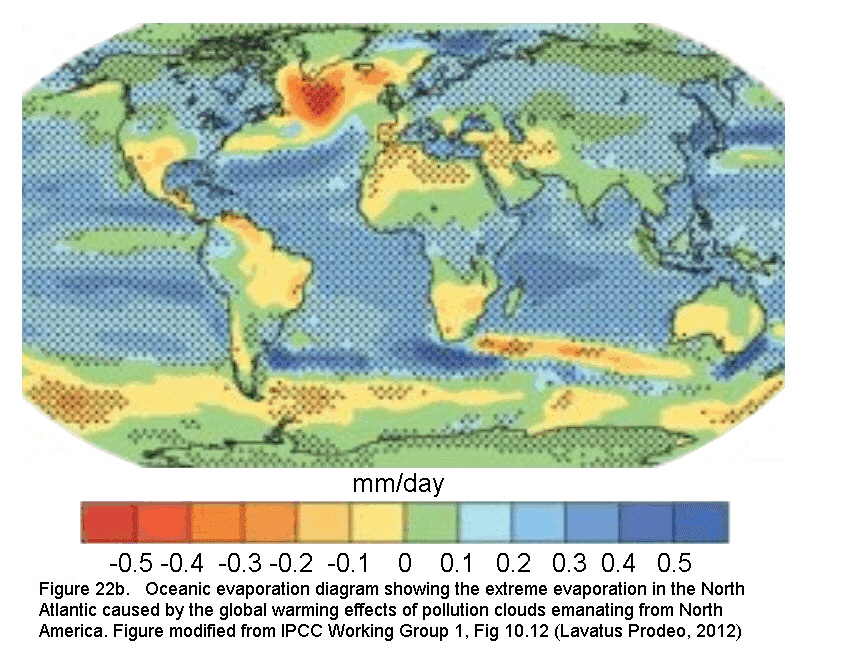
The normal high July temperatures of the Arctic ocean region including the major heated rivers feeding the surrounding Siberian shelf regions are an important factor in destabilization of the shallower methane hydrate accumulations and the eruption of methane into the Arctic atmosphere and stratosphere at that time (Shakova et al. 2008, 2010; Light 2012). In the normal July summer hot period the Gulf Stream is heated to some 26.5 degrees C in the Atlantic (Figure 22a,b). This has been found to be followed by a subsequent anomalous hot period in late October - November caused by the high global warming potential of methane clouds which have been erupted into the Arctic atmosphere and make their way up into the global stratosphere (Figure 23). The stratospheric build up of methane between about 30 km and 47 km altitude forms a continuous methane global warming veil which is then spread by stratospheric vortices ESE across Russia, Europe the Atlantic and the Americas into the Pacific and Southern Hemisphere where it enhances both the pollution heated Gulf Stream on the east coast of the United States/Canada and the El-Nino in the Pacific (Figure 23). This secondary thermal anomaly caused by the extreme methane eruptions in late October - November is termed a False Indian Summer (FIS) and it will grow in strength, depth and duration as the methane eruptions escalate exponentially in the Arctic emission centres because of the increased heating of the subsea methane hydrates by the summer warmed Gulf Stream (Intermediate Depth) current (Figures 19, 20a,b and 22a,b).
The stratospheric methane global warming veil completes a complex convection cycle in the earths atmosphere and oceans in exactly the same way that a giant forest fire will draw in cooler winds which will amplify the flames with the heated air rising, cooling and increasing in density aloft so that it sinks back to the ground away from the fire site to be drawn back again to re-enhance the flames further. In the case of the Gulf Stream where global warming induced by the pollution clouds blowing off the east coast of the United States/Canada warms the Atlantic waters in the summer to 26.5 degrees C (Figure 22b), the heat is then trapped in the Gulf Stream which migrates north east to the Arctic in October November where it destabilizes the subsea methane hydrates along the south east slope of the Eurasian basin/Laptev Sea transition and forms an extreme atmospheric methane eruption centre (Figure 20a,b).
The US/Canada pollution clouds which globally overheat the Gulf Stream also show a second complete complex energy convection cycle caused by a southern offshoot
of the Gulf Stream in the Atlantic that swings SE toward the warm waters of the western coast of Africa, the spawning grounds of Hurricane systems in the Eastern Atlantic (Wales, 2012). These hurricanes then make their way to the NW towards the Gulf Coast/Florida, the source of the warmed Gulf Stream, causing increasing devastation on their way across the Caribbean islands and the US/Canada coastline. Both the stratospheric methane global warming veil and the Hurricane tracks are simply the closing stages of complex heat convection cycles returning back to the original energy source (the pollution clouds blowing off the east coast of the US/Canada) increased volumes of heat energy. The global warming effects of these pollution clouds will be enhanced even further by methane being injected into the Arctic atmospheric convection cycles producing an escalating exponential growth in the heat input into atmosphere and ocean, intensifying the resulting climatic devastation and giving us an early warming of our impending extinction within the next 50 years.
Introduction
The Arctic sea ice maintains the cold of the polar region and acting like the Earth's air conditioner it helps moderate the climate with the oceans and the atmosphere rebalancing the heat on the planet (Rice 2012; Speer 2012). Each year the Arctic sea ice melts in the summer reaching its smallest extent in September and reaches it largest extent in March (Rice 2012). At the end of August 2012, the Arctic sea ice reached it lowest extent that has ever been recorded (Vizcarra, 2012) due to the increasing input of globally warmed Gulf Stream waters into the Arctic causing what is now termed a death spiral for the Arctic floating ice field (Romm 2012; Morison 2012). In the IPCC fourth assessment report in 2007 it was predicted that the Arctic would become ice free at the end of this Century, while more recent estimates suggest that the ice would melt by 2030 or in this decade (Romm 2012). Projections based on Piomas ice volume melt data show that by 2015 the floating Arctic ice cap will be gone (Carana 2012d; Masters, 2009) and this paper confirms the accuracy of that estimate.
During early analysis of the global Giss surface temperature data in the Arctic it was discovered that very high Giss atmospheric surface temperature anomalies appeared in November and an analysis was made using only the November data for the entire data set (1951 to 2011) from which a maximum Arctic methane atmospheric thermal gradient was calculated (Light 2011). This Arctic November Giss thermal gradient was found to closely match an Arctic atmospheric thermal gradient determined from the 11 year moving average of the Gakkel Ridge earthquake data calibrated to the ratio of the normal global IPCC thermal gradient and 11 moving average of the progressive growth of Normal and Major Earthquakes with magnitudes greater than seven (Light 2011). Subsequently the entire global monthly mean Giss surface temperature data set has been investigated in detail from 1951 to 2012 by recording the mean maximum global Giss surface temperature achieved for every month from 1951 to 2012 on the NASA Goddard Space Flight Center polar plots of the Earths surface temperature (NASA 2012).


The 12 month (yearly) moving average trend of the maximum Giss monthly maximum surface temperature anomalies are shown on Figure 2 (NASA 2012). The sharp peak in 1957 is again probably due to methane degassing of methane hydrates in the slope areas around Antarctica. Both the 12 month (yearly) and 11 year moving averages of the Giss maximum global surface temperature anomalies show identical trends overlapping almost perfectly and this does not add any more information to the interpretation (Figure 3). The mean exponential trend from the increase in the Giss maximum global surface temperature anomalies rises from around 5.5 degrees C in 1965 to more than 7 degrees C by 2022. The 1.5 degrees C temperature increase is probably from increasing but erratic release of methane from the Arctic (Figure 3).

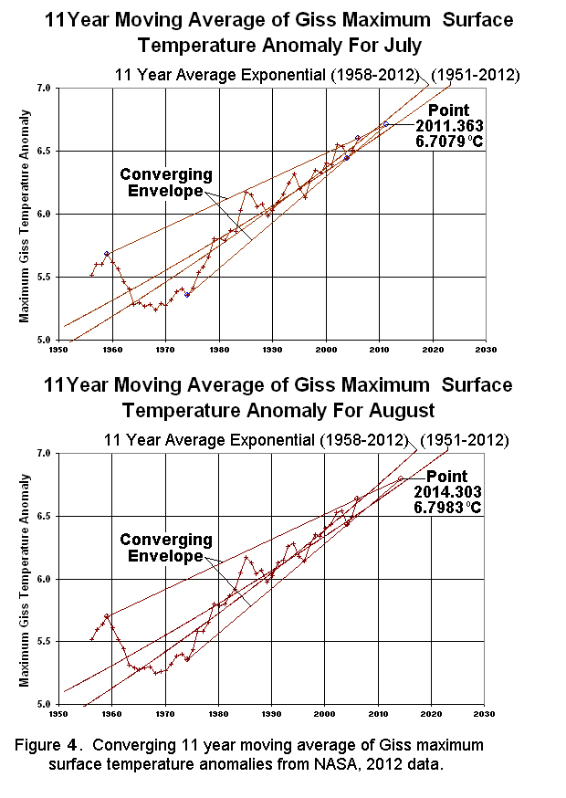


The mean exponential trends for the higher (1958 - 2012) monthly global 11 year Giss maximum surface temperature data set which largely eliminates the early Antarctic heat anomaly as well as the mean exponential trend for the lower full data set from (1951 - 2012) are also shown on all of the 12 graphs (Figures 4 to 9).


The same error field is shown in Figure 12 as in Figure 11 onto which two mean exponential gradients have been plotted which very closely bracket the final mean convergent amplitude point at 2015.757. These two exponential curves have been constructed by finding the mean of the September 11 year moving average and the October 11 year moving average for the two ranges (1958 - 2012) and (1951 - 2012). It is clear that these two exponential lines for September and October pass very close to the mean convergent amplitude intersection point at 2015.757 which has a calculated date of October 2nd 2015. This further confirms that we are looking at true seasonal data and probably a correct estimate of the time for the complete melt back of the floating Arctic ocean ice cap. The September and October exponential gradients are also closely parallel to the maximum temperature gradient estimated using the two most extreme end points (July and June) on Figure 11.


Figure 15 shows the close correlation between the Piomas exponential estimate of the volume melt back time of the Arctic sea ice cap in 2015, the 12 month mean estimate of the Arctic sea ice loss at 2015.757 and the Greenland ice sheet exponential reduction in reflectivity from melting by 2014 (Light 2012; Carana 2012d; Carana 2012c). The Greenland ice sheet now shows an exponential decrease in its reflectivity (albedo) from surface melting which reached values below 66.5% in 2011 (after Box and Decker 2011 with exponential projection by Carana 2012c).
 |
| (click to enlarge) |
From 2015 (see Figure 15) the sea level is calculated to rise at an increased rate after Arctic sea ice melt back and the Arctic ocean will absorb large quantities of heat because of the sharp reduction in reflectivity of the dark open ocean surface and exponentially increasing rates of emission of high global warming potential methane into the atmosphere from destabilized subsea Arctic methane hydrates (see Figure 18, left blue line calibrated to sea level rise)(Light 2012; Dessus et al. 2008).
Figure 15 also shows the global sea level (GSL) anomaly curve after correction for reservoir impoundment water from 1900 - 2007 (Chao, Yu and Li 2008). The global sea level rise is 2.46 mm/year over the period 1930 to 2007 (Chao, Yu and Li 2008). From the start of October 2015 the dark Arctic ocean will be completely open to the sun and absorb large quantities of heat and this heat absorption will be accelerated exponentially because the ice front will no longer be cooling the increasingly hot Gulf Stream where it enters the Arctic west of Svalbard and migrates up the slope of the Eurasian basin to the extreme subsea atmospheric methane eruption centre at the transition to the Laptev Sea. The sea level will then rise at an increased rate of some 15.18 cm/year from 2015 to 2017 reaching a maximum depth of 68.3 metres (Wales 2012) in 2051 (Light 2012). This is a 100% lose - lose situation for humanity and for all life on Earth.

 Figure 16 and Table 2 show the change in the relative mean monthly methane global warming potentials calculated from the intersection points of the converging amplitude envelopes of the monthly eleven year moving average of the Giss maximum surface temperature data. The mean monthly methane global warming potentials drop sharply from 500 for July (Summer through Autumn, Winter and Spring) to 55.4 for June at the end of Spring (Figure 16; Table 2). Figure 16 has been derived by overlaying the error field of the intersection points (see Figure 11) of the 12 monthly converging amplitude envelopes of the 11 year moving average of the Giss maximum surface temperatures (NASA 2012) onto the atmospheric methane global warming potential field (GWP) derived from Svalbard methane concentration data (Light 2012).
The two major opposing excursions that occur in the error graph (Figure 16) around the 21st of September (Autumn) equinox and the 21st of March (Spring) equinox indicate as previously stated that the mean monthly maximum surface temperature data is showing a true seasonal relative variation and is not a result of some random errors in the data set. A final mean methane yearly global warming potential of 119.39 was determined from the mean intersection points of the 12 converging amplitude envelopes of the monthly 11 year moving average of the maximum Giss surface temperatures (NASA 2012) and is situated in mid winter on Figure 16. Summer and Autumn have methane global warming potentials greater than 124 (Figure 16). The methane global warming potential is found to fall sharply from April to June from above 100 to 54.4 around the time of the March 21 Spring equinox during a period of lengthening days (Figure 16; Table2). Quite clearly the increasing day length and solar heating should in fact be increasing the global warming potential of the methane because of increasing methane concentrations, so the factor controlling the falling methane GWP will need to be sought elsewhere.

The straight line temperature trend of the 2012 Arctic Barrow methane anomaly (Carana 2012), the mean absolute maximum Giss exponential trend (which overlaps the 8 degrees C anomaly total deglaciation line), the mean atmospheric 2 degrees C anomaly line and the 500 methane global warming potential line for Svalbard outline an extinction zone in yellow through which the methane enhanced global atmospheric temperature gradient is most likely going to pass. The global ice cap air surface temperatures are seen to lag behind the fast rising atmospheric temperatures because of local cooling by the solid ice (Light 2012). Figure 17 also shows the Piomas 2015 estimate of the time of melting of Arctic sea ice (Carana 2012d) and the estimate of the Arctic sea ice melt time of 2015.76 from the mean of the 12 intersection points of the monthly converging amplitude envelopes of the 11 year moving averages of the maximum Giss surface temperatures (NASA 2012). The range of the determined methane global warming potentials on Figure 17 is seen to extend from near 50 to 500.

The Arctic Intermediate Depth Current
A detailed 3D picture of the warm Arctic (2 degrees C maximum temperature) Intermediate Depth current which is an extension of the warm Gulf Stream in the Arctic is shown in Figure 19. The globally warmed Gulf Stream begins its journey off the East Coast of the United States and enters the Arctic Ocean and Eurasian basin west of Svalbard.

Gas Reserves in the Arctic Region
The Norwegian and Arctic Basins have some 1000000 square kilometres (1*10^ 12 square metres) of slopes exposed to the warm Gulf Stream (Intermediate Depth ) current with an average potential thickness of some 450 metres (Light 2012; Light and Solana 2002 a; Kholodov et al., 2001). The Arctic methane hydrate reserves will be estimated by taking account that of the fact that of the mean subsea methane hydrate thickness of 450 metres, only 200 metres are in contact with the Intermediate Depth current (300 m to 500 m depth range) and are being destabilized (Light and Solana 2002 a,b). We can therefore use 450 metres and 200 metres as two end members of a reserve estimate with the mean lying near 325 metres.
Each cubic metre of gas hydrate contains some 164 cubic metres of methane gas so the total reserves of the Norwegian and Arctic Basins are estimated at ranging from 3.28*10^16 to 7.38*10^16 cubic metres of methane with a mean value of 5.33*10^16 cubic metres of methane (Light and Solana, 2002 a).
Giant gas fields are required to have more than 3*10^12 cubic feet (8.5*10^10 cubic metres) of ultimately recoverable gas (Halbouty, 2001). The calculated range of gas reserves for the methane hydrates in the Norwegian and Arctic basins is equivalent to a range of 386 to 868 thousand giant gas fields with a mean near 627 thousand giant gas fields. Thus Arctic subsea methane can form a giant green energy gas resource for humanity for the next several hundred years during the transition to sustainable energy resources (Light 2012).
The normal high July temperatures of the Arctic ocean region including the major heated rivers feeding the surrounding shelf regions are an important factor in destabilization of the shallower methane hydrate accumulations and the eruption of methane into the Arctic atmosphere and stratosphere at that time (Shakova et al. 2008, 2010). The methane hydrates on the East Siberian shelf occur at much shallower depths of 50 metres or less and these are much more vulnerable to rising water temperatures caused by fresh water fluxes in the summer introduced by coastal rivers and by the effects of Atlantic current systems in the Arctic (Shakova et al. 2008, 2010; Romm 2012). The methane hydrate reserves of the East Siberian shelf are estimated at 1.4*10^12 tonnes of methane (Shakova et al. 2010).
The Gulf Stream
Although the Gulf Stream has been known since the 1500's (Figures 20a,b; 21; 22a,b) (Wales 2012), the global heating of the western Gulf Stream due to the effects major pollution clouds blowing of the east coast of the United States/Canada is a more recent phenomenon causing a region of extreme evaporation in the Summer and the heating of the Atlantic water to 26.5 degrees C (The reddish zone on Figures 22a,b). Increase in the size of the pollution clouds blowing off the east coast of the Unites States/Canada has led to an increase of some 1 degree C in the temperature of the warm Gulf Stream (Arctic Intermediate Depth) current where it dives beneath the Arctic ice pack towards the pole west of Svalbard (Figures 20a,b and 22a,b). The total distance covered from west of Miami on the east coast of the United States/Canada to the extreme methane eruption centres at the Eurasian basin/Laptev Sea transition is between 12 400 to 12 500 km. This current comes in contact with the methane hydrates at a depth of some 300 metres along the south eastern slope of the Eurasian Basin before it runs aground on the methane hydrate rich slope of the Gakkel Ridge at the transition to the Laptev Sea, a zone of extreme atmospheric methane eruptions (Figures 20a,b and 21)(Light 2012, Light and Solana 2002 a,b; Wales, 2012)

Arctic Intermediate Depth Current as an Extension of Warm Gulf Stream
Although the Gulf Stream has its origins west of Florida, it is only north of Miami along the east coast of the United States/Canada and in the Atlantic where it is subjected to the greatest evaporation from global warming induced by pollution clouds blowing eastwards off the continental US/Canada and where it first achieves anomalously high temperatures (Figures 22a, b, the reddish region). The wind driven north east trending Gulf Stream is shrouded by the polluted air and grows in width and heat across the Atlantic until it baths the western shores of Europe. A section of the Gulf Stream passes north of Scotland and west of Norway where it splits into two currents, one to the east which flows into the Barents Sea (Yermack branch) and the other to the west (Svalbard branch) swings passed the west side of Svalbard as the West Spitsbergen Current (Figure 20a,b)(Wales 2012; Boyd and Dasaro 1994). The West Spitsbergen current is a warm (5 degrees C to 8 degrees C) salty (ca 35 psu) current, some 100 km wide flowing at about 0.35 m/sec toward the polar regions (Figure 20) (Wales 2012; Boyd and Dasaro 1994). The flow rate of the warm Gulf Stream (West Spitsbergen Current) fluctuates from 20 million cubic metres/second (20 sverdrups) in February in mid winter and decreases to 5 million cubic metres/second (5 sverdrups) in August in the high summer (Figure 20)(Fahrbrach et al. 2001).
West of Svalbard the warm Gulf Stream current maintains its oceanic salinity (ca 35 psu; Aagaard et al. 1987) but it is cooled by the cold Polar atmosphere and the increase in density makes the core of the current sink to some 300 meters (total depth range 5 to 500 metres) to form the "Lower Arctic Intermediate Current " (Figure 19 and 20, Light and Solana 2002 a,b). The density of the "Lower Intermediate Current" increases and it sinks beneath a surface layer of fresher water caused by the melting of the front of the sea ice pack which is driven back up to 400 km in a narrow lead by the strong warm western branch of the Gulf Stream (Figure 20a,b)(West Spitsbergen Current - Boyd and Dasaro 1994). The eastern Yermack branch of the warm Gulf Stream current enters a zone of strong tidal mixing in the Barents Sea where it forms a warm moderately saline mixture with the Polar waters only 300 metres deep similar to the depth of the return Atlantic East Greenland Current (Figure 20a,b)(Bourke et al. 1988; Manley 1995).

The Arctic extension of the Gulf Stream, the "Arctic Intermediate Depth Current" remains relatively warm and is very saline (ca 35 psu)(Dmitrenko et al. 2008) and it forms a completely isolated unit from the fresher waters generated by the melting of the frontal zone of the Arctic ice pack mixed with fresh water run off from fjords in Northern Svalbard (Figure 20a,b) (Boyd and Dasaro 1994; Saloranta et al. 2001). Large amounts of ice are encountered by the warm Gulf Stream (West Spitsbergen current) along the continental shelves of Svalbard and the warm Gulf Stream waters sink at a much faster rate due to the increased quantities of fresh water melt from the sea ice (Figure 20a,b)(Haugan 1999). The faster rate of sinking of the warm Gulf Stream beneath the fresh water melt means that it retains a larger amount of its heat which is not lost to the surrounding waters or atmosphere (Figure 20a,b)(Haugan 1999). These anomalously warm waters are transported directly into the Arctic where they are destabilizing the methane hydrates at the extreme methane eruption zones on the continental slope (Figure 20a,b)(Light and Solana 2002 a,b) on the eastern end of the Eurasian Basin/Gakkel Ridge/Laptev Sea. The warm Arctic Intermediate Depth current is thus a major cause of Arctic sea ice melting (Haugan 1999) because of the global warming effects of the large volumes of methane released into the atmosphere from the destabilized methane hydrates(Light 2011, 2012).

By 2008, the core temperature of the warm Gulf Stream intermediate depth current (300 metres depth) had increased by some 1 degrees C (Wales 2012; Aagaard 1987) where it is in direct contact with the top of the stability zone of the methane hydrates leading to their destabilization and the release of methane to the ocean and atmosphere (Figure 19) (Light and Solana 2002 a,b) The decrease in the core temperature of the warm Gulf Stream (Intermediate Depth Current) at some 300 metres depth as it migrates cyclonically around the Arctic from the west of Svalbard means that it is loosing heat to the surrounding slope methane hydrates destabilizing them and to the enclosing water causing increased Arctic sea ice melting (Figure 19)(Light and Solana 2002 a,b; Aagaard et al. 1987; Westbrook et al. 2009).
North of the New Siberian Islands the warm Intermediate Depth current (Gulf Stream) runs aground in a region where there is a large zone of methane hydrate accumulations on the slope and where the shelf edge suddenly swings westward closing the Eurasian Basin at the Laptev Sea transition (Figure 20a,b). It is here that it is progressively destabilizing the subsea methane hydrates and releasing increasingly large volumes of methane into the Arctic atmosphere at an exponential rate (Figure 20a,b)(Light 2011, 2012) . This is also where the easterly and shallower (base 300 metres) Yermack Branch of the warm Gulf Stream, that had entered the Barents Sea, flows above the main grounded Gulf Stream (Intermediate Depth) current forming an extensive zone of shallower massive methane hydrate destabilization on the shelf (Figure 20a,b). The Yermack branch of the Gulf Stream intersects shallower methane hydrates to the south east (50 metres depth or less) where the warm Gulf Stream appears to be destabilizing the methane hydrates to a slightly lesser extent and causing widespread zones of atmospheric methane emissions (Figure 20a,b).
The warm (ca 2 degrees C) Gulf Stream (Intermediate Depth) current with a strong Atlantic chemical signature is then cyclonically recirculated in the Arctic basin bringing it in contact with many other zones of shelf/slope methane hydrates (Light 2011; 2012) and it reaches depths of 400 to 500 metres at the Beaufort Gyre before it is pushed out of the Arctic as the shallower East Greenland Current (Figure 20a,b)(Dmitrenko et al 2008; Perkin and Lewis 1984). However throughout the Arctic the Gulf Stream Intermediate Depth current still retains a weak Atlantic chemical signature (Saloanta et al 2001).

There is a very close correlation between the extreme zones of atmospheric methane emissions in the Arctic and the distribution of subsea methane hydrates (Figure 21 after Max and Lowrie, 1993; Shakova et al 2012; AIRS methane data from Saldo 2012). There is a strong relationship between the slope methane hydrate deposits at the end of the Eurasian Basin/Laptev sea transition and extensive extreme subsea atmospheric methane emission zones (torches) which over lie them. A clear link also exists between the subsea atmospheric methane emission zones and methane overpressured shear and normal fault systems caused by the slow wedge like opening of the Arctic Gakkel ocean ridge (Light 2012; Harrison et al 2008). The widespread destabilization of the methane hydrates caused by the increasing rate of earthquake activity along the Gakkel Ridge and heating by the warm Gulf Stream (Arctic Intermediate Depth) current all have their origin in the pollution clouds blowing off the North American continent and initially generating massive heating and evaporation in the Atlantic Gulf Stream (22a,b).
The stratospheric methane global warming veil completes a complex convection cycle in the earths atmosphere and oceans in exactly the same way that a giant forest fire will draw in cooler winds which will amplify the flames with the heated air rising, cooling and increasing in density aloft so that it sinks back to the ground away from the fire site to be drawn back again to re-enhance the flames further. In the case of the Gulf Stream where global warming induced by the pollution clouds blowing off the east coast of the United States/Canada warms the Atlantic waters in the summer to 26.5 degrees C, this heat is then trapped in the Gulf Stream which migrates north east to the Arctic in October -November where it destabilizes the subsea methane hydrates along the south east slope of the Eurasian basin and forms an extreme atmospheric methane eruption centre at the transition to the Laptev Sea (Figure 20a,b).
The Arctic methane because of its low density (about half that of air at standard temperature and pressure) rises vertically like hydrogen into the stratosphere where it forms a continuous methane global warming veil at an altitude of some 30 km to 47 km (Figure 23)(Light 2012; Engineering Toolbox 2011). This methane global warming veil is then spread by stratospheric vortices ESE back via Russia, Europe, the Atlantic and the United States/Canada to the Pacific where it enhances the global heating of both the Gulf Stream to the East and El Nino to the west of North America (Figure 22a,b and 23) (Light 2012). The stratospheric methane global warming veil is adding more energy back to the Gulf Stream off the east coast of the US/Canada in exactly the same way that the marginal winds drawn into a forest fire help to enhance its fury.

The US/Canada pollution cloud globally warmed Gulf Stream also shows a second complete complex energy convection cycle caused by a southern offshoot in the Atlantic which swings SE to warm waters of the western coast of Africa which happens to be the spawning grounds of Hurricane systems in the Atlantic (Wales, 2012). These hurricanes then make there way to the NW toward the Gulf Coast/Florida, the source of the Gulf Stream causing increasing devastation on their way across the Caribbean island chain and the US/Canada coastline. Both the stratospheric methane global warming veil and the Hurricane tracks are simply the closing stages of complex heat convection cycles returning back to the original energy source (the pollution clouds blowing off the east coast of the United States/Canada) with increased volumes of heat energy. The global warming effects of the pollution clouds are being continually enhanced even further by methane being injected into the Arctic Stratospheric methane global warming veil producing an escalating exponential growth in the heat input into atmosphere and ocean and intensifying the resulting climatic devastation.
Implications of the Transfer of Gulf Stream Heat to the Arctic Methane Hydrates
A direct consequence of the approximate 3.9 month delay in the transfer of heat from the pollution heated region of the east coast of the United States/Canada to the extreme methane eruption zones at the east end of the Eurasian Basin/Laptev Sea transition is that the weather systems of the Northern Hemisphere will now begin to develop a secondary thermal peak in late October - November which will grow in size as the stratospheric methane concentrations increase due to the exponential growth of methane eruptions in the Arctic (Figures 20a,b, 21 and 22a,b).
The normal July summer hot period in the Atlantic, in which the Gulf Stream is heated to some 26.5 degrees C will be followed by a subsequent anomalous hot period in late October to November due to the high global warming potential of methane clouds which have been erupted into the Arctic atmosphere and then made their way into the stratosphere (Figure 23). The stratospheric build up of methane between about 30 km and 47 km altitude forms a continuous methane global warming veil which is spread by stratospheric vortices ESE across Russia, Europe the Atlantic and North America into the Pacific where it enhances both the pollution heated Gulf Stream on the east coast of the United States/Canada and the El-Nino in the Pacific (Figures 22a,b and 23).
An Indian summer is a heat wave that occurs in the Autumn in the Northern Hemisphere between late September and mid November (Wales, 2012). Indian summers usually occur after a killing frost and have above normal temperatures and dry and hazy conditions (Wales, 2012). Anomalous heating in October was first clearly observed in Southern Spain in October 2011 without any preceding freezing temperatures and upset the normal pattern of Mediterranean winter rains, causing widespread drought and wild fire problems. The sudden appearance of this heating correlates well with the effects of the start of exponential methane release recorded in the Arctic at Svalbard in August 2010 which produced a later heating of the earths atmosphere because of its high global warming potential (Light 2011, 2012; Carana 2011). The growth of this second thermal anomaly during late October and November due to the effects of Arctic methane release in the Northern Hemisphere can be ascribed to the effects of summer pollution clouds pouring off the east coast of the United States/Canada globally warming the Gulf Stream waters on their way to the methane hydrate destabilization grounds in the subsea Arctic (Figures 20a,b, 21 and 22a,b).
This secondary thermal anomaly caused by the extreme Arctic methane eruptions in late October - November will be termed a False Indian Summer (FIS) and it will grow in strength, depth and duration as the methane eruptions escalate exponentially in the Arctic emission centres because of the increased heating of the subsea methane hydrates by the summer warmed Gulf Stream (Intermediate Depth) current (Figures 19, 20a,b, 21 and 22a,b).
From the sequence of Gulf Stream heating and cooling and the resulting methane emission events in the Arctic it is possible to roughly predict how the future weather system is going to alter. The northern hemispheres summer year will consist of normal summer heat in July (Relative methane GWP = 500 ) a period of slightly cooler conditions in August - September (Figure 16) (Relative methane GWP from 161 to 133.6). This will be followed by a False Indian Summer (FIS) between October and November with sharply increased relative methane GWP's between 187.3 to 177.7 during a period of extreme methane emission from the Arctic methane emission centres (Figure 16). Because the FIS occurs after a long summer it will be marked by extreme dryness, drought conditions and a high probability of uncontrollable wildfires as well as extreme weather conditions (Hurricanes and Tornadoes). The Northern Hemisphere winter period (December to February) will also be marked by increased methane eruptions because this now represents the arrival time of heated Gulf Stream waters at the Arctic methane eruption centres that were warmed off the east coast of the United States/Canada by the preceding False Indian Summer between October and November (Figures 20a,b, 21 and 22a,b).
During the winter, the relative methane global warming potential falls from 167.9 to 109.9 although this is a period of increasing day length after the shortest day (December 21)(Figure 16). After the March 21 spring equinox the day length continues to increase during spring until the June 21st when the relative methane global warming potential falls to its lowest value of 54.4 (Figure 16). This period of reduced methane emission from the Arctic methane emission zones is caused by the fact that the Gulf Stream waters sourced from the east coast of the United States/ Canada were strongly cooled during the winter weather systems between December, January and February and they are the ones that arrived at the Arctic methane eruption centres from April to June. Consequently the relative methane global warming potential calculated from the Giss surface temperature data falls off sharply from 103.1 in April to 54.4 in June by the time the longest day arrives and the first day of summer occurs on June 21st (Figure 16, NASA 2012).
Conclusions
The normal high July temperatures of the Arctic ocean region which includes the major heated rivers feeding the surrounding shelf regions are an important factor in destabilization of the shallower methane hydrate accumulations and the eruption of methane into the Arctic atmosphere and stratosphere at that time (Shakova et al. 2008, 2010).
During the False Indian Summer (October - November) we can view the excessive summer global warming of the Gulf Stream off the east coast of the United States/Canada as a direct result of the effects of eastward migrating pollution clouds pouring off the US/Canada coast. This heat is transferred by the Gulf Stream directly to the most extreme methane eruption centres at the end of the Eurasian Basin in the Arctic in October - November where the release of methane to the atmosphere and stratosphere generates a sequence of events that returns more heat back to the source zone on the North American continent. The arrival of the stratospheric methane warming veil over North America causes massive heating and drying, extensive droughts, uncontrollable wildfires and extreme hurricane and tornado events in the following summer.
We can look on the globally heated Gulf Stream as the United States/Canadian pollution hot line to climatic hell. Unless the United States/Canada undertake a immediate extreme reduction in their carbon dioxide output of some 80% by converting all their oil and coal based power stations and industries to natural gas or renewable energy sources, all ground and air transport systems to natural gas, ethanol and electricity, the climatic pain will continue to get more and more severe and the recovery cost become astronomical.


The Lucy proposal is a radio beat frequency system for destroying the first hydrogen bond in atmospheric methane when it forms dangerously thick global warming clouds over the Arctic (Figure 25)(Light and Carana). It generates similar gas products to those normally produced by the natural destruction of methane in the atmosphere over some 15 to 20 years. This system will use similar frequencies to those used in generating nano-diamonds from methane gas in commercial applications over the entire pressure range of the atmosphere from the surface to 50 km altitude (Light and Carana, 2012). The environmental group of Rockwell International is researching Lucy as a viable option for destroying methane clouds within the Arctic atmosphere and in other regions (Hensel pers. com. 2012).
The French/German Lidar stratospheric methane detecting satellite Merlin should be launched as soon as possible (scheduled for 2014 - Ehret 2010) to give early warning of the build up of methane in the stratospheric global warming veil (Figure 23). A methane detecting Lidar system should also be immediately installed on the International Space Station to detect methane in the 30 km to 47 km altitude, methane global warming veil in the stratosphere and act as a back up and calibration for the Merlin satellite (Figure 23).
The UN/US must immediately declare an international emergency of the most extreme kind and call for a conference of world governments and oil companies to select the fastest and most efficient way to deal with the Arctic methane eruption threat. We are already two years past the tipping point in August 2010 when massive subsea atmospheric methane eruptions started in earnest in the Arctic. The next three years are all we have left to try to put a break on the Arctic methane emissions before the heating effects and sea level rise due to loss of Arctic sea ice and Arctic methane induced global warming will be completely unstoppable and humanity will be facing total extinction before the middle of this Century (2050).
REFERENCES
Aagaard K., Foldvik A., Hillman S.R., 1987. The West Spitsbergen Current: Disposition and Water Mass Transformation. Journal of Geophysical Research 92:3778
Allen, P.A., and Allen, J.R. 1990. Basin Analysis, Principles and Applications. Blackwell, Oxford, 451 pp.
Anitei S. 2007. How is the Ozone layer menaced? The Daily Climate. www. Daily Climate.org
http://news.softpedia.com/news/How-is-the-Ozone-Layer-Menaced-53762.shtml
ARCTIC METHANE EMERGENCY GROUP
http://arctic-methane-emergency-group.org
Bourke R.H., Wiegel A.M. and Paquette R.G. 1988. The westward turning branch of the West Spitsbergen Current. Jounal of Geophysical Research 93: 14065 - 14077
Box J. and Decker D. 2012. Greenland Ice Sheet Reflectivity , July 2000 – 2011, 2012 days 1 – 23. NASA MOD1OA1 data processed by Jason Bird and David Decker. Byrd Polar Research Centre. Projection in red added by Sam Carana, 2012.
Boyd T.J. D'asaro E.A., 1994. Cooling the West Spitsbergen Current: Wintertime
Observations West of Svalbard. Journal of Geophysical Research 99:22587
Calder, N. 1984. Timescale - An Atlas of the Fourth Dimension. Chatto and Windus,
London, 288 pp.
Carana, S. 2011a. Runaway Warming 2011. Geo-engineering blog
http://geo-engineering.blogspot.com/2011/09/runaway-warming.html
Carana S., 2011b. Runaway global warming, 2011. Geo-engineering blog
http://geo-engineering.blogspot.com/2011/04/runaway-global-warming.html
Carana, S. 2011c. Light, M.P.R. and Carana, S. 2011c. In Arctic-News: Methane linked to seismic activity in the Arctic.
http://arctic-news.blogspot.com.au/p/seismic-activity.html
Carana, S. 2012a. Striking increase of methane in the Arctic. In: Arctic News
http://arctic-news.blogspot.com/2012/05/striking-increase-of-methane-in-arctic.html
Carana S., 2012b. Record levels of greenhouse gases in the Arctic. Arctic News. Wednesday, May 2, 2012.
http://arctic-news.blogspot.com/2012/05/record-levels-of-greenhouse-gases-in.html
Carana S., 2012c. Greenland is melting at incredible rate. Arctic News.
http://arctic-news.blogspot.com/2012/07/greenland-is-melting-at-incredible-rate.html
Carana S., 2012d. Getting the picture. Arctic News.
http://arctic-news.blogspot.com/2012/08/getting-the-picture.html
Chao, B.F., Yu, Y.H., Li, Y.S., 2008. Impact of Artificial Reservoir Water Impoundment on Global Sea Level. Science, v. 320, p. 212 – 214.
http://www.skepticalscience.com/sea-level-rise.htm
Church J.A., White N.J., Thorkild A., Wilson W.S., Woodworth, P.L. Domingues C.M., Hunter J.R., Lambeck K., 2008. Understanding global sea levels: past, present and future. Special Feature. Original Article. Sustain Sci. V.3, pp. 9 - 22.
http://academics.eckerd.edu/instructor/hastindw/MS1410_001_FA08/handouts/2008SLRSustain.pdf
Coachman L.K. and Barnes C.A., 1963. The movement of the Atlantic water in the Arctic Ocean. Arctic, 16(1); 9 - 16.
Dessus, B., and Laponche B., Herve le Treut, 2008. Global Warming: The Significance of Methane bd-bl-hlt January 2008.
http://www.global-chance.org/IMG/pdf/CH4march2008.pdf
Dmitrenko I.A., Polyakov I.V., Kirilov S.G., Timokhov L.A., Frolov I.E., Sokolov V.T., Simmons H.L., Ivanov V.V., et al. 2006. Toward a warmer Arctic Ocean: Spreading of the early 21st Atlantic Water warm anomaly along the Eurasian Basin margins. Journal of Geophysical Research 113: C05023
Edwards, M. H., Kurras, G. J., Toltsoy, M., Bohnenstiehl, D. R., Coakley, B. J., Cochran, J. R., 2001. Evidence of recent volcanic activity on the ultraslow – spreading Gakkel ridge. Letters to nature. Nature 409. no.6822, 808 – 812.
http://www.volcano.si.edu/world/volcano/cfm?vnum=1707-02-&volpage=var
Ehret G. 2010. Merlin: French – German Climate Satellite to be launched in 2014. Lidar Department, Institute of Atmospheric Physics, Deutches Zentrum für Luft – und Raumfahrt (DLR)
http://www.dlr.ge/pa/en/desktopdefault.aspx/tabid-2342/6725_read-26662/
Engineering Toolbox, 2011. Gases – Specific Gravities.
http://www.engineeringtoolbox.com/specific-gravities-gases-d_334.html
Fahrbach E., Meincke J., Osterhus S., Rohardt G., Schauer U., Tverberg V., Verduin J., 2001. Direct measurements of volume transports through Fram Strait. Polar Research 20(2), 217
Galt J.A. 1967. Current Measurements in the Canadian Basin of the Arctic Ocean, Summer, 1965. Technical Report No.184. Arctic Institute of North America. Office of Naval Research.
https://dlib.lib.washington.edu/dspace/bitstream/handle/1773/16076/M67-15.pdf?sequence=1
Harrison, J.C., St-Onge, M.R., Petrov, O., Streinikov, S., Lopatin, B., Wilson, F., Tella, S., Paul, D., Lynds, T., Shokalsky, S., Hults, C., Bergman, S., Jepsen, H. F. and Solli, A., 2008. Geological Map of the Arctic, Geological Survey of Canada, Open File 5816, Scale 1:1000,000. 5 Sheets. Arctic Map on Adobe Illustrator:
http://gscof-5816-e-2008-mn01.pdf
Halbouty M. 2001. Giant Oil and Gas Fields of the Decade (1990 - 1999). An Introduction:
http://www.searchanddiscovery.com/documents/halbouty03/index.htm
Hargraves, 2012. Altitudes of World Cities. Hargraves Advanced Fluidic Solutions.
http://www.hargravesfluidics.com
Haugan P. M., 1999. Structure and heat content of the West Spitzbergen Current. Polar Research 18 (2), 183
Heicklen, J. 1976. Atmospheric Chemistry. Academic Press, New York, 406 pp.
Hillen, M.H., Jonkman, S.N., Kanning, W., Kok, M., Geldenhuys M., Vrijling J.K. and Stive, M.J.F., 2010. Coastal Defence Cost Estimates Case Study of the Netherlands, New Orleans and Vietnam. The Netherlands, TU Delft. Available from:
http:/tiny.cc/wikh
IPCC Fourth Assessment Report on Climate Change 2007 - temperature rise projections
http://ipcc.ch/publications_and_data/ar4/wg1/en/spmsspm-projections-of.html
IPCC (2007), Fourth Assessment Report, FAQ 3.1, Figure 1 (WG1, Ch 3, p. 253)
http://www.ipcc.ch/pdf/assessment-report/ar4/wg1/ar4-wg1-chapter3.pdf
Intergovernmental Panel on Climate Change (IPCC) 1992a. Climate Change. The IPCC Scientific Assessment (Edited by J. J. Houghton, G. J. Jenkins and J. J. Ephraums). Cambridge University Press, Cambridge. U.K.
Intergovernmental Panel on Climate Change (IPCC) 1992b. Climate Change in 1992. The Supplementary report to the IPCC Scientific Assessment (Edited by J. J. Houghton, B. A. Callander and S. K. Varney). Cambridge University Press, Cambridge. U.K.
Intergovernmental Panel on Climate Change (IPCC) 2007a. Fourth Assessment Report on Climate Change 2007. FAO 3.1, Figure 1, WG1, Chapter 3, p. 253.
http://blogs.ei.colombia.edu/wp-content/uploads/2010/12/graph-2-600X422.jpg
Intergovernmental Panel on Climate Change (IPCC) 2007b. Synthesis Report
http://www.ipcc.ch/publications_and_data/ar4/syr/en/spms1.html
Kvenvolden K.A. 1988. Methane hydrate - a major reservoir of carbon in the shallow geosphere? - Chemical Geology, v.71, pp.41 - 51.
Kvenvolden, K. A., and Lorenson, T. D., 2001. The global occurence of natural gas hydrate. In: C. K. Paul and W. P. Dillon (Eds.). Natural Gas Hydrates. Occurence, distribution and detection.
Geophysical Monograph 124. American Geophysical Union. p. 3 - 18.
Lavatus Prodeo 2012. Living in a 4C World.
Lavatusprodeo.net/archives/2010/08/16/living-in-a-4C-world
Kholodov , A.I., Romanovskii N.K., Gavrilov A.V., Tipenko, G.S., Drachev S.S., Hubberten H.W., Kassens H., 1999. Modeling of the Offshore Permafrost Thickness on the Laptev Sea Shelf. Polarforschung 69, 221 - 227.
Lide. D.R. and Frederikse H.P.R., 1995. CRC Handbook of Chemistry and Physics. 75th Edition, CRC Press, London. pp. 1-1 - 1-33.
Light M.P.R. 2011a. Use of beamed interfering radio frequency transmissions to decompose Arctic atmospheric methane clouds. Edited by Sam Carana.
http://arctic-news.blogspot.com/p/decomposing-atmospheric-methane.html
Light M.P.R. 2011c. Stratospheric methane global warming veil. Edited by Sam Carana. In: Arctic News.
http://arctic-news.blogspot.com.au/p/stratospheric-methane-global-warming.html
Light M.P.R., 2012a. Global exctinction within one human lifetime as a result of a spreading atmospheric methane heatwave and surface firestorm. Edited by Sam Carana. In Arctic News.
http://arctic-news.blogspot.com/p/global-extinction-within-one-human.html
Light M.P.R., 2012b. How much time is there left to act, before methane hydrate
releases will lead to human extinction? Edited by Sam Carana. In: Geo-Engineering.
http://geo-engineering.blogspot.com/2012/02/how-much-time-is-there-left-to-act.html
Light M.P.R. 2012c. Angels Proposal - A Proposal for the Prevention of Arctic Methane Induced Catastrophic Global Climate Change by Extraction of Methane from beneath the Permafrost/Arctic Methane Hydrates and its Storage and Sale as a Subsidized "Green Gas" Energy Source. LGS. 49 pp. In: Arctic News.
http://arctic-news.blogspot.com.es/2012/05/proposal-to-extract-store-and-sell.html
Light, M.P.R. et al., 2011b. Methane linked to seismic activity in the Arctic
http://arctic-news.blogspot.com/p/seismic-activity.html
Light M.P.R. and Solana C., 2002a. Arctic methane hydrates - Mapping a potential greenhouse gas hazard. Abstract and Poster, EGS, Nice. - Appendix at:
http://arctic-news.blogspot.com/p/seismic-activity.html
Light, M.P.R. and Solana, C. , 2002b- Arctic Methane Hydrates: A Potential Greenhouse Gas Hazard
http://adsabs.harvard.edu/abs/2002EGSGA..27.4077L
Lopatin, N.V. 1971. Temperature and geologic time as factors in coalification (in Russian). Akad. Nauk SSSR. Izvestiya. Seriya Geologicheskaya, 3, pp.95 - 106.
Manley T.O. 1995. Branching of the Atlantic Water within the Greenland-Spitsbergen
Passage. An estimate of recirculation. Journal of Geophysical Research 100: 20627
Masters. J. 2009. Top Climate Story of 2008. Arctic Sea Ice Loss. Dr Jeff Masters Wunderblog.
http://www.wunderground.com/blog/JeffMasters/comment.html?entrynum=1177
Max, M.D. & Lowrie, A. 1993. Natural gas hydrates: Arctic and Nordic Sea potential. In: Vorren, T.O., Bergsager, E., Dahl-Stamnes, A., Holter, E., Johansen, B., Lie, E. & Lund, T.B. Arctic Geology and Petroleum Potential, Proceedings of the Norwegian Petroleum Society Conference, 15-17 August 1990, Tromso, Norway. Norwegian Petroleum Society (NPF), Special Publication 2 Elsevier, Amsterdam, 27-53.
Merk J. 2012. CPSP118G Spring Semester SGC Colloquim. Climate and How it Works I. Physical Components. University of Maryland.
http://www.geol.umd.edu/sgc/lectures/climatepart1.html
MIT. 2012. Mission 2011. Saving the Oceans. Climate Change
http://web.mit.edu/12.000/www/M2011/finalwebsite/solutions/climate.shtml
Morison 2012. Sea Ice Death Spiral Driving Atlantic Water into Arctic Causing Wild Weather. Get Energy Smaart! Now. Blogging for a Sustainable Energy Future.
http://getenergysmartnow.com/2012/01/20/sea-ice-death-spiral-driving-atlantic-water-into-arctic-causing-wild-weather/
Nassar R., Bernath P.F., Boone C.D., Manney G.L., McLeod S.D., Rinsland C.P., Skelton R., Walker K.A., 2005. Stratospheric abundances of water and methane based on ACE-FTS measurements. Geophysical Research Letters, Vol. 32, LI5504, 5 pp.
http://www.atmosp.physics.utoronto.ca/~rnassar/Publications_pdfs/Nassar_water_methane_2005GL022383.pdf
NASA global temperature data
http://data.giss.nasa.gov/gistemp/tabledata_v3/GLB.Ts.txt
NOAA 2011a. Huge sudden atmospheric methane spike Arctic Svalbard (north of - Norway)
http://arctic-news.blogspot.com/p/need-for-geo-engineering.html
NOAA 2011b. Huge sudden methane spike recorded at Barrow (BRW), Alaska, United States. Generated ESRL/GMO – 2011. December 14-17-21 pm
http://arctic-news.blogspot.com/p/need-for-geo-engineering.html
NSIDC, 2011a. The Polar Vortex. National Snow and Ice Data Center.
http://nsidc.org/arcticmet/patterns/polar_vortex.html
Olivier C.P. 1942. Long Enduring Meteor Trains. Proc. Amer. Phil. Soc. 35, 93.
Olivier C.P. 1948. Long Enduring Meteor Trains. Proc. Amer. Phil. Soc. 91, 315 (Second paper).
Parry, M.L., Canziani, O.F., Palutikof, J.P. and Co-authors, 2007. Impacts, Adaption and Vulnerability. Contribution of Working Group II to the Fourth Assessment Report of the Intergovernmental Panel on Climate Change. M.L. Parry, O.F. Canziani, J.P. Palutikof, P.J. van der Linden and C.E. Hanson, Eds. Cambridge University Press, Cambridge, UK, pp. 23 – 78.
Perkin R.G. and Lewis F.I. 1984. Mixing in the West Spitsbergen Current. Journal of
Physical Oceanography 14 (8), 1315
Reynold N. 2012. Methane hydrate technology fuels a new energy regime.
http://www.methanehydrate.org
Rice D., 2012. Arctic Sea Ice at Lowest Level on Record. Sci-Tech Today. Environment.
www.sci-tech-today.com/story.xhtml?story_id=130007AH6NIG
http://www.methanehydrates.org
Romm J. 2012. Why the Arctic Sea Ice Death Spiral Matters. Think Progress - Climate Progress.
thinkprogress.org/climate/2012/08/26/745571/why-the-arctic-sea-ice-death-spiral-matters
http://www.methanehydrates.org
Saldo R. 2012. AIRS data. DTU Space, Technical University of Denmark.
http://www.seaice.dk
Saloranta T.M., Svendsen H. 2001. Across the Arctic front west of Spitsbergen. High-resolution CTD sections from 1998 - 2000. Polar Research 20 (2). 177. 1751 - 8369.
Science Daily, 2011. Record Depletion of Arctic Ozone Layer Causing Increased UV Radiation in Scandinavia.
http://www.sciencedaily.com/releases/2011/04/110405102202.htm
Semiletov, I. 2011. Quoted from Itar-Tass. Heavy methane emissions found in the Arctic Eastern Sector. Itar-Tass. September 26, 2011.
http://www.itar-tass.com/en/c154/233799.html
Shakova N., Semiletov, I., Salyuk, A., and Kosmach, D., 2008. Anomalies of methane in the atmosphere over the East Siberian Shelf. Is there any sign of methane leakage from shallow shelf hydrates?
EGU General Assembly 2008. Geophysical Research Abstracts, 10, EGU2008-A-01526
http://www.cosis.net/abstracts/EGU2008/01526/EGU2008-A-01526.pdf
Shakova, N. and Semiletov, I., 2010a. Methane release from the East Siberian Shelf and the potential for abrupt climate change. Presentation in November 30, 2010.
http://symposium2010.serdp-estcp.org/Technical-Sessions/1A
Shakova N., Semiletov, I., Leifer, I., Salyuk, A., Rekant, P., and Kosmach, D. 2010b.
Geochemical and geophysical evidence of methane release over the East Siberian Arctic Shelf. Journal Geophys. Research 115, C08007
http://europa.agu.org/?view=article&uri=/journals/jc/jc1008/2009jcoo5602/2009jc005602.xml
Shakova, N., Semiletov, I., Salyuk, A., Yusupov, V., Kosmach, D., and Gustafsson, O., 2010c.
Extensive methane venting to the atmosphere from sediments of the East Siberian Arctic Shelf. Science.
http://www.sciencemag.org/content/327/5970/1246.short
Speer K. 2012. How ocean currents affect global climate is a question oceanographers may be close to awnsering. Florida State University.
http://www.eurekalert.org/pub_releases/2012-08/fsu-hoc082612.php
http://www.methanehydrates.org
Tharp. M., and Frankel, H., 1986. In: Natural History, October 1986. North American Museum of Natural History, p. 1 – 6.
http://www.google.es/url?.sa=t&rt
University of Washington 2000. "North pole Hydrography 1991 - 2000 compared with EWG Atlas Climatology". EWG Atlas 1950's. Oden 1991. Scicex 1993-1999.
North Pole Environmental Observatory 2000. Cast 18.
Vizcarra N. 2012. Arctic Sea Ice Reaches Lowest Extent Ever Recorded. University of Colorado CU- Boulder Research Team.
http://www.eurekalert.org/pub_releases/2012-08/uoca-asi082712.php
http://www.methanehydrates.org
Wofsy, S.C. et al. 2009. (image: HIPPO-1 flight along the date line, January 2009)
HIAPER Pole-to-Pole Observations (HIPPO): fine-grained, global-scale measurements of climatically important atmospheric gases and aerosols Phil. Trans. R. Soc. A (2011) 369, 2073–2086 doi:10.1098/rsta.2010.0313
http://rsta.royalsocietypublishing.org/content/369/1943/2073.full.html
Wales J. 2012. Wikipedia
Carbon Dioxide. http://en.wikipedia.org/wiki/Carbon_dioxide
Climate of the Arctic. http://en.wikipedia.org/wiki/climate_of_the_Arctic
Density of Air. http://en.wikipedia.org/wiki/Density_of_air
Global Warming. http://e.wikipedia.org/wiki/Global_warming
Gulf Stream. http://en.wikipedia.org/wiki/Gulf_stream
Iceberg. http://en.wikipedia.org/wiki/Iceberg
Indian Summer. http://en.wikipedia.org/wiki/Indian_summer
Methane. http:/en.wikipedia.org/wiki/Methane
Natural Gas. http:/en.wikipedia.org/wiki/Natural Gas
North Sea. http:/en.wikipedia.org/wiki/North_Sea
Enthalpy of Fusion. http://en.wikipedia.org/wiki/Enthalpy_of_fusion
Jason-1. http://en.wikipedia.org/wiki/jason-1
Current Sea Level Rise. http://en.wikipedia.org/wiki/Current_sea_level_rise
West Spitsbergen Current. http://en.wikipedia.org/wiki/West_Spitsbergen_Current
Westbrook G.K., Thatcher K.E., Rohling E.J., Pitrowski A.M., Palike, H., Osborne A.H., Nisbet E.G., Minshuli, T.A. et al. 2009. Escape of methane gas from the seabed along the West Spitsbergen continental margin.
Geophysical Research Letters 36 (15). L15608.
Yurganov, L., 2012a. Atmospheric Infrared Sounder (AIRS) data from NASA's Aqua Satellite. Index of/pub/yurganov/methane/MAPS/
ftp://asl.umbc.edu/yurganov/methane/MAPS/
Yurganov, L., 2012b. Atmospheric Infrared Sounder (AIRS) data from NASA's Aqua Satellite.
ftp://asl.umbc.edu/pub/yurganov/methane/AIRS_CH4%20_2002-2012.jpg
No comments:
Post a Comment