Wednesday, November 25, 2020

There is no time to lose

Carbon dioxide levels continue at record levels, despite COVID-19 lockdown, the WMO reports. The increase in carbon dioxide from 2018 to 2019 was larger than that observed from 2017 to 2018 and larger than the average annual growth rate over the last decade.

The rise has continued in 2020. The lockdown did cut emissions of many pollutants and greenhouse gases, but any impact on carbon dioxide levels - the result of cumulative past and current emissions - is in fact no bigger than the normal year to year fluctuations. 

“Carbon dioxide remains in the atmosphere for centuries and in the ocean for even longer. The last time the Earth experienced a comparable concentration of CO₂ was 3-5 million years ago, when the temperature was 2-3°C warmer and sea level was 10-20 meters higher than now. But there weren’t 7.7 billion inhabitants,” said WMO Secretary-General Professor Petteri Taalas.

“The COVID-19 pandemic is not a solution for climate change. However, it does provide us with a platform for more sustained and ambitious climate action to reduce emissions to net zero through a complete transformation of our industrial, energy and transport systems. The needed changes are economically affordable and technically possible and would affect our everyday life only marginally. It is to be welcomed that a growing number of countries and companies have committed themselves to carbon neutrality,” he said. “There is no time to lose.”


Above image illustrates the steep rise in methane, compared to carbon dioxide and nitrous oxide. Levels of carbon dioxide, methane and nitrous oxide reached new highs in 2019, reports the WMO. Carbon dioxide (CO₂) rose to 410.5 ppm (148% of its pre-industrial level), methane (CH₄) to 1877 ppb (260% of pre-industrial) and nitrous oxide (N₂O) to 332.0 ppb (123% of pre-industrial).

So, given that there's no time to lose, why mention carbon neutrality, and not 100% clean, renewable energy? Also, let's not lose sight of other emissions such as N₂O. Yes, dramatic cuts in CO₂ emissions do need to happen rapidly, and yes, this does require a complete transformation of industry, energy and transport. Nonetheless, N₂O emissions are also important and most N₂O emissions result from land use, such as food production and waste handling, which must also change. 

[ from earlier post ]
The IPCC (AR5) gave N₂O a lifetime of 121 years and a 100-year global warming potential (GWP) of 265 times that of carbon dioxide. Furthermore, N₂O also causes stratospheric ozone depletion. 

The IPCC, in special report Climate Change and Land, found that agriculture, forestry and other land use activities accounted for some 13% of CO₂, 44% of CH₄, and 82% of N₂O emissions from human activities globally during 2007-2016, representing 23% of total net anthropogenic emissions of greenhouse gases.

If emissions associated with pre- and post-production activities in the global food system are included, the emissions could be another 14% higher, i.e. as high as 37% of total net anthropogenic greenhouse gas emissions, the IPCC added.

Let's get back to that 23%. The IPCC calculates this 23% by using a GWP of 28 for CH₄. Over the first few years, however, the GWP of CH₄ is more than 150, as discussed in an earlier post. When using a GWP of 150, land use emissions rise from 23% to 31%, as the image on the right shows. Add another 14% from further food-related emissions and the total share for land use becomes 45% of people's emissions. 

[ click on images to enlarge ]
In other words, all polluting emissions need to be reduced. Moreover, a recent paper by Jorgen Randers et al. points out that, even if all greenhouse gas emissions by people could stop immediately and even if the temperature anomaly could fall to 0.5°C above pre-industrial, greenhouse gas levels would start rising again after 2150 and keep rising for centuries to come. Another recent paper, by Tapio Schneider et al., points out that solar geoengineering may not prevent strong warming from direct effects of CO₂ on stratocumulus cloud cover. 

This means that the threat is even more menacing when including large methane releases that threaten to occur as temperatures keep rising in the Arctic and sediments at the seafloor of the Arctic Ocean threaten to get destabilized, resulting in the eruption of huge amounts of methane. 

What is the joint impact of carbon dioxide and methane? The WMO reported CO₂ levels of 410.5 ppm and CH₄ levels of 1877 ppb in 2019. As discussed in an earlier post, over the first few years after release, methane's GWP is more than 150 times higher than carbon dioxide. Accordingly, the 2019 level of 1877 ppb of methane translates into global heating of 281.55 ppm CO₂e. Together, that makes 692.5 ppm CO₂e, which is 507.5 ppm CO₂e away from the 1200 ppm CO₂e cloud tipping point

The image below illustrates that the joint impact of carbon dioxide and methane could cause the 1200 ppm CO₂e tipping point to be crossed in 2040. The image uses IPCC and WMO through 2019 to display three lines, with added trends: 
- Black line: CO₂ in parts per million (ppm);
- Red line: CH₄ in ppm CO₂e, using a GWP of 150;
- Purple line: CO₂ and CH₄ in ppm CO₂e.

Trends for CH₄ are selected to reflect a steep rise as a result of methane hydrate destabilization. 

How could such a steep rise in methane levels occur?

Stronger methane releases from subsea permafrost can be expected, says a paper by Natalia Shakhova et al. A 1000-fold methane increase could occur, resulting in a rise of as much as 6°C within 80 years, with more to follow after that, according to a paper by Atsushi Obata et al.

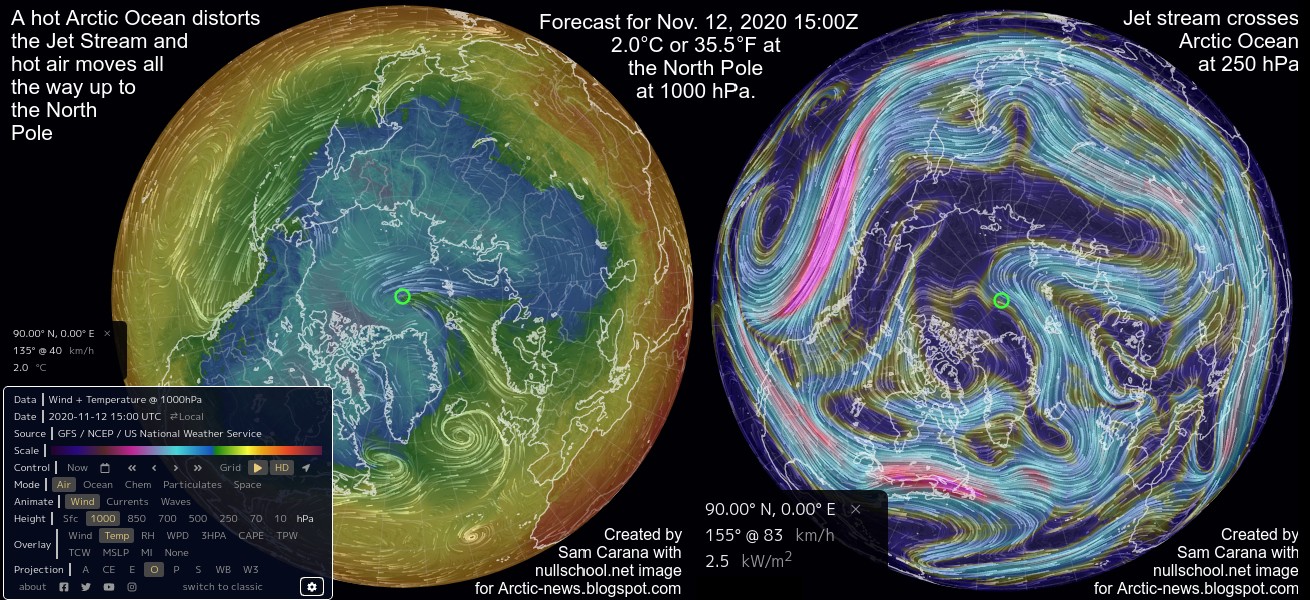
Seafloor methane releases could be triggered by strong winds causing an influx of warm, salty water into the Arctic ocean (see this earlier post and this page). 

Since little hydroxyl is present in the atmosphere over the Arctic, it is much harder for this methane to get broken down.

Even relatively small methane releases could cause tremendous heating, if they reach the stratosphere.

Methane rises from the Arctic Ocean concentrated in plumes, pushing away the aerosols and gases that slow down the rise of methane elsewhere, which enables methane erupting from the Arctic Ocean to rise straight up fast and reach the stratosphere. 

The IPCC (AR5) gave methane a lifetime of 12.4 years. The IPCC (TAR) gave stratospheric methane a lifetime of 120 years, adding that less than 7% of methane did reach the stratosphere at the time.

The images on the right illustrate this. On November 20 pm, 2020, the MetOp-1 satellite recorded high methane levels over the Arctic Ocean at 293 mb (top image on the right). This corresponds with an altitude of some 9 km altitude, which is where the Stratosphere starts at the North Pole. The global mean methane level at that altitude was 1921 ppb.

The next images show areas with high levels of methane, as indicated by the magenta color, remaining present over the Arctic Ocean even at higher altitudes.

The higher the altitude, the more methane will concentrate over the Equator. Yet at 229 mb, high methane levels are still visible north of Siberia, while global mean methane levels were still very high, i.e. 1916 ppb. 

Even at 156 mb, there still are high methane levels visible (green circle, third image right). 

The conversion table shows that the Tropopause, which separates the Troposphere from the Stratosphere, is lower over the North Pole (at about 9 km altitude) than over the Equator (17 km altitude). 

The fifth image on the right, from an earlier post, shows that methane has accumulated more at higher altitudes over the years. 

The sixth image on the right shows that the MetOp-1 satellite recorded mean methane levels of 1925 ppb at 293 mb on December 2, 2020 am, with high methane levels present over the Arctic Ocean.

The next image shows that a peak methane level of 2715 ppb was recorded by the SNPP satellite on November 30, 2020 pm at 399.1 mb.

The animation on the right shows high methane levels recorded by the MetOp-2 satellite on December 2, 2020 pm, at a number of altitudes: 

- At 1000 mb (close to ground/sea level) a peak methane level of 2129 ppb shows up north of Svalbard. 

- At 918 mb, methane peaks at 2408 ppb and high methane levels show up over the Artic Ocean.

- At 815 mb, methane reaches a peak of 2582 ppb and high methane levels are visible over larger parts of the Arctic Ocean. 

- At 742 mb, methane reaches a peak of 2663 ppb and high methane levels are visible over even larger parts of the Arctic Ocean. 

- At 586 mb, methane reaches a peak of 2518 ppb and high methane levels are visible over a huge part of the Arctic Ocean, while hardly any high levels of methane are visible over land. 

- At 293 mb, methane reaches a peak of 2411 ppb and high levels of methane are still visible over the Arctic Ocean, even at this high altitude. 

[ from earlier post ]
In conclusion, a huge temperature rise could occur soon, even with a relatively small increase in carbon dioxide and methane releases. 

As above image illustrates, a temperature rise of more than as 10°C could eventuate as soon as 2026 when taking into account aerosol changes, albedo changes, water vapor, nitrous oxide, etc., as an earlier analysis shows. 

The joint impact of these warming elements threatens the cloud tipping point to be crossed and the resulting 8°C rise would then come on top of the 10°C rise, resulting in a total rise of 18°C, as illustrated by the image on the right, from an earlier post.

Indeed, there is no time to lose. It is high time to stop the denial of the size of the threats and challenges that the world faces, the harm inflicted and the speed at which developments could strike. 

The situation is dire and calls for immediate, comprehensive and effective action, as described in the Climate Plan


• WMO Greenhouse GasBulletin
https://public.wmo.int/en/resources/library/wmo-greenhouse-gas-bulletin

• WMO news release: Carbon dioxide levels continue at record levels, despite COVID-19 lockdown
https://public.wmo.int/en/media/press-release/carbon-dioxide-levels-continue-record-levels-despite-covid-19-lockdown

• Understanding the Permafrost–Hydrate System and Associated Methane Releases in the East Siberian Arctic Shelf, by Natalia Shakhova, Igor Semiletov and Evgeny Chuvilin (2019)
https://www.mdpi.com/2076-3263/9/6/251

• Damage of Land Biosphere due to Intense Warming by 1000-Fold Rapid Increase in Atmospheric Methane: Estimation with a Climate–Carbon Cycle Model - by Atsushi Obata et al. (2012) 
https://journals.ametsoc.org/doi/full/10.1175/JCLI-D-11-00533.1

• Possible climate transitions from breakup of stratocumulus decks under greenhouse warming, by Tapio Schneider et al. (2019)
https://www.nature.com/articles/s41561-019-0310-1

• Solar geoengineering may not prevent strong warming from direct effects of CO2 on stratocumulus cloud cover - by Tapio Schneider et al. 
https://www.pnas.org/content/early/2020/11/10/2003730117

• An earth system model shows self-sustained thawing of permafrost even if all man-made GHG emissions stop in 2020 - by Jorgen Randers et al.
https://www.nature.com/articles/s41598-020-75481-z


Monday, November 16, 2020

Accelerated global warming and stadial cooling events: IPCC oversights regarding future climate trends

 by Andrew Glikson

The linear nature of global warming projections by the IPCC (2014) Assessment Report (AR5) (Figure 1) appears to take little account of stadial cooling events, such as have followed peak temperature rises in previous interglacial stages. The linear trends appear to take only limited account of amplifying positive feedback effects of the warming from land and ocean. A number of factors cast doubt on IPCC climate change projections to 2100 AD and 2300 AD, including:
Figure 1 (a) IPCC average surface temperature change to 2100 relative to 1986-2005 IPCC AR5;
(b) IPCC average surface temperature change to 2300 relative to 1986-2005 IPCC AR5

However, global temperature measurements for 2015-2020 indicate accelerated warming due to both the greenhouse effect reinforced by a solar radiation maximum (Hansen and Sato 2020) (Figure 2).

Figure 2. Accelerated Global Warming reinforced by both greenhouse 
gases and a solar maximum Hansen and Sato, 2020

The weakening of the northern Jet stream, due to polar warming and thus reduced longitudinal temperature contrasts, allows penetration of warm air masses into the polar region and consequent fires (Figure 3). The clash between tropical and polar air and water masses (Figure 3A) leads to regional storminess and contrasting climate change trajectories in different parts of the Earth, in particular along land-ocean boundaries and island chains. 

The weakening of the jet stream and migration of climate zones constitute manifestations of an evolving Earth’s energy imbalance¹, namely a decrease in reflection of solar radiation from Earth to space and thereby global warming. Earth retained 0.6 Watt/m² during 2005-2010 and 0.87 Watt/m² during 2010-2020 (Hansen and Sato 2020), primarily due to a rise in greenhouse gases but also due to a solar radiation peak. During 2015-2020 global warming rates exceeded the 1970-2015 warming rate of 0.18°C/per decade, a deviation greater than climate variability. Hansen and Sato (2020) conclude the accelerated warming is caused by an increasing global climate forcing, specifically by the role of atmospheric aerosols.

Figure 3 A. Undulating and weakening jet stream and the polar vortex and penetration
of warm air, inducing Arctic warming and fires.     B. Satellite images of Wildfires
ravaging parts of the Arctic
, with areas of Siberia, Alaska, Greenland and Canada
engulfed in flames and smoke. While wildfires are common at this time of year, record-
breaking summer temperatures and strong winds have made 2020 fires particularly bad.

Bronselaer et al., 2018 modelled a meltwater-induced cooling of the southern hemisphere toward the end 21st century by as low as -1.5°C (Figure 4A). Hansen et al. 2016 estimated the time frame of 21st century stadial cooling event as dependent on the rates of ice melt (Figure 4B), reaching near global extent toward the end of the century (Figure 4C).

Figure 4 A. 2080–2100 meltwater-induced sea-air temperature anomalies relative to
the standard RCP8.5 ensemble (Bronselaer et al., 2018). Hatching indicates where the
anomalies are not significant at the 95% level;  B. Negative temperature anomalies
through the 21st-22nd centuries signifying stadial cooling intervals (Hansen et al., 2016);
C. A model of Global warming for 2096, where cold ice melt water occupies large parts
of the North Atlantic and circum-Antarctica, raises sea level by about 5 meters and
decreases global temperature by -0.33°C (Hansen et al., 2016).

With the concentration of greenhouse gases rising by approximately 47% during the last century and a half, faster than almost any observed rise in the Cenozoic geological record, the term “climate change” refers to an extreme shift in state of the atmosphere-ocean system. The greenhouse gas rise and temperature rise rates are faster than those of the K-T mass extinction, the Paleocene-Eocene extinction and the last glacial termination.

The consequences for future climate change trends include:
  • Further expansion of the tropical climate zones and a polar-ward shift of intermediate climate zones, leading to encroachment of subtropical deserts over fertile Mediterranean zones. 
  • Spates of regional to continent-scale fires, including in Brazil, Siberia, California, around the Mediterranean, Australia.
  • A weakened undulating jet stream (Figure 3) allowing penetration of and clashes between warm and cold air and water masses, with ensuing storms. 
  • In Australia the prolonged drought, low vegetation moisture, high temperatures and warm winds emanating from the northern Indian Ocean and from the inland, rendering large parts of the continent tinder dry and creating severe fire weather subject to ignition by lightning.
  • The delayed melting of the large ice sheets due to hysteresis², would be followed by sea level rise to Pliocene levels, ~25 meters above pre-industrial levels, once sea level reaches equilibrium with temperature of 2 to 3 degrees Celsius or higher, changing the geography of the continents.
It would follow from these considerations that succeeding periods of peak temperatures, extensive melting of the ice sheets, flow of ice melt into the oceans and thereby stadial cooling would lead to clashes between tropical fronts and cooling masses of air, producing storminess, in particular along continental margins and island chains. The modelled time frame of these developments (Figure 4B) may be cyclical, or may extend further in time and place as long as the ice sheets continue to breakdown.


¹ Earth's energy imbalance is the difference between the amount of solar energy
absorbed 
by Earth and the amount of energy the planet radiates to space as heat.
If the imbalance is 
positive, more energy coming in than going out, we can expect
Earth to become warmer in t
he future — but cooler if the imbalance is negative.
² Hysteresis is the dependence of the state of a system on its history. For example the 
melting of an ice sheet may occur slowly depending on its previous state.

Andrew Glikson

Dr Andrew Glikson
Earth and Paleo-climate scientist
ANU Climate Science Institute
ANU Planetary Science Institute
Canberra, Australia


Books:
The Asteroid Impact Connection of Planetary Evolution
http://www.springer.com/gp/book/9789400763272
The Archaean: Geological and Geochemical Windows into the Early Earth
http://www.springer.com/gp/book/9783319079073
Climate, Fire and Human Evolution: The Deep Time Dimensions of the Anthropocene
http://www.springer.com/gp/book/9783319225111
The Plutocene: Blueprints for a Post-Anthropocene Greenhouse Earth
http://www.springer.com/gp/book/9783319572369
Evolution of the Atmosphere, Fire and the Anthropocene Climate Event Horizon
http://www.springer.com/gp/book/9789400773318
From Stars to Brains: Milestones in the Planetary Evolution of Life and Intelligence
https://www.springer.com/us/book/9783030106027
Asteroids Impacts, Crustal Evolution and Related Mineral Systems with Special Reference to Australia
http://www.springer.com/us/book/9783319745442


Wednesday, November 11, 2020

Above Zero Celsius at North Pole November 2020

Above image shows that, in October 2020, the Arctic Ocean was very hot. The Copernicus image below shows temperatures averaged over the twelve-month period from November 2019 to October 2020.

Keep in mind that, in the Copernicus image, anomalies are compared to the 1981-2010 average.

Note that the shape of the recent twelve-month period is similar to the 2016 peak, when there was a strong El Niño, while in October 2020 the temperature was suppressed due to La Niña and due to low sunspots.

The image below shows how a hot Arctic Ocean distorts the Jet Stream and hot air moves all the way up to the North Pole. 

Above image shows the Northern Hemisphere at November 12, 2020, with a temperature forecast of 2.0°C or 35.5°F at the North Pole at 1000 hPa at 15:00Z. On the right, jet stream crosses the Arctic Ocean (at 250 hPa). At surface level, a temperature was forecast to be 0.6°C or 33.2°F. 


As it turned out, the highest temperature at the North Pole was 1.1°C or 34.1°F on November 12, 2020, at 1000 hPa at 18:00Z, as above image shows. At 15:00Z that day, a temperature of 1.9°C or 35.3°F was recorded at 1000 hPa just south of the North Pole, at 89.50° N, 1.50° E.

The image below shows temperature anomalies for November 12, 2020, with forecasts approaching 30°C. 


[ Click on images to enlarge ]
These high temperatures over the Arctic Ocean are caused by transfer of huge amounts of heat from the Arctic Ocean to the atmosphere, indicating severe overheating of the Arctic Ocean as a result of the ongoing movement of ocean heat at the surface of the North Atlantic to the Arctic Ocean along the Gulf Stream. 

As the image on the right shows, temperature anomalies above 20°C were recorded over a large part of the Arctic Ocean on November 16, 2020. 

As illustrated by the image below, temperature anomalies are forecast to remain high over the Arctic Ocean, with the forecast for November 26, 2020, showing anomalies approaching 30°C. 


The resulting distortion of the Jet Stream can at times speed up winds that move hot air from the North Atlantic Ocean toward to Arctic Ocean, as illustrated by the image at the top. 

[ click on images to enlarge ]
The image on the right shows that the Jet Stream was as fast as 411 km/h or 255 mph south of Greenland (at the green circle), before crossing the Arctic Ocean on November 4, 2020. 

The image below shows how, on November 20, 2020 15:00 UTC, a distorted Jet Stream reaches a speed of 327 km/h or 203 mph (at circle, globe left). At 850 hPa, wind reaches speeds as high as 161 km/h or 100 mph (circle, globe right). 

The danger is that such strong wind will speed up ocean currents in the North Atlantic that carry huge amounts of heat toward the Arctic Ocean. 


The image below shows sea surface temperature anomalies compared to 1981-2011 on the Northern Hemisphere on October 23, 2020, when anomalies off the coast of North America were as high as 10.8°C or 19.5°F (left), and on December 3, 2020, when anomalies off the coast of North America were as high as 12.7°C or 22.8°F (right). 


According to a recent news report, an atmospheric river smashed into Juneau, Alaska, dropping 5.08 inches of rain in 24 hours ending 3 a.m. Wednesday December 2, 2020.

This is not an isolated event, but a symptom of the unfolding catastrophe referred to as global warming, which threatens to remove all life from Earth.

Sea surface temperatures around North America are very high. The above image shows that sea surface temperatures were as much as 12.7°C or 22.8°F higher than 1981-2011 off the east coast of North America on December 3, 2020 (green circle). On the image below, the globe on the left shows that sea surface temperature anomalies (SSTA) were as high as 4.1°C or 7.3°F off the west coast of North America on December 4, 2020 (at the green circle).

These high sea surface temperatures speed up de Jet Stream over oceans. At this time of year, temperatures over continents are low, so there is greater ocean/land temperature difference, which further speeds up the Jet Stream where it travels over oceans toward continents. The center globe shows wind as fast as 381 km/h or 237 mph at the time (at circle). 

At the same time, the narrowing temperature difference between the Equator and the North Pole is slowing down the Jet Stream. This is making the Jet Stream more wavy at higher latitudes, even resulting in circular wind patterns, and this can make a lot of cold air leave the Arctic and move over continents, thus further widening the ocean/land temperature difference. Given that more than 90% of global warming goes into oceans, this is an important self-reinforcing feedback of global warming. 

Stronger wind results in stronger evaporation, which cools down the sea surface somewhat, as the blue areas over the Pacific Ocean indicate. Due to the strong wind, much of the moisture falls down farther on the path of the wind. The globe on the right shows 3-hour precipitation accumulation as high as 31.3 mm or 1.23 in off the west coast of North America (green circle). 


The image below shows an earlier analysis, describing the situation in September 6, 2020, when high sea surface temperatures on the Northern Hemisphere and a narrow difference between the Equator and the North Pole distorted the Jet Stream, making it cross the Arctic Ocean, form circular wind patterns and reach speeds as fast as 262 km/h or 163 mph (250 hPa, green circle) over the North Atlantic. The globe on the right shows that the Gulf Stream off the North American coast reached speeds of 8 km/h or 5 mph (at green circle). 

[ click on images to enlarge ]

More ocean heat can move into the Arctic Ocean for a number of reasons, including: 
  • At times, the Jet Stream becomes very strong and elongated over the North Atlantic, speeding up the flow of ocean heat along the path of Gulf Stream all the way to the Arctic Ocean;
  • Overall, winds are getting stronger, speeding up ocean currents running just below the sea surface;
  • Stratification of the North Atlantic results in less heat mixing down to lower parts of the ocean; and 
  • Increased evaporation and increased subsequent rainfall farther down the path of the Gulf Stream forms a colder freshwater lid stretched out at the sea surface from the North Atlantic to the Arctic Ocean, sealing off transfer of heat from ocean to atmosphere and consequently moving more heat just underneath the sea surface into the Arctic Ocean.

    [ from earlier post ]
As the image below shows, sea surface temperatures as high as 16.6°C or 61.9°F were recorded north of Svalbard on November 9, 2020. 


As the image below shows, the N2O satellite recorded a peak methane level of 2762 ppb on the morning of November 16, 2020.


As the image below shows, the MetOp-1 satellite recorded a peak methane level of 2725 ppb on the afternoon of November 18, 2020.


The video below shows a methane plume or bubble cloud spotted by a team of 69 scientists from ten countries documenting bubble clouds rising from a depth of around 300 metres (985ft) along a 150km (93 mile) undersea slope in the Laptev Sea.


The danger is that even more hot and salty water will reach the shallow parts of the Arctic Ocean that contain huge amounts of methane in the form of hydrates and free gas in sediments at the seafloor, resulting in huge eruptions of methane that, on its own, could almost instantly cause the 1200 ppm CO₂e cloud feedback tipping point to be crossed, which can cause global temperatures to rise by 8°C.

Latent heat loss, feedback #14 on the Feedbacks page

The situation is dire and calls for comprehensive and effective action, as discussed in the Climate Plan.


Links

• Climate Plan
https://arctic-news.blogspot.com/p/climateplan.html

• NASA GISS Surface Temperature Analysis - global maps

• Copernicus - surface air temperature for October 2020

• Climate Reanalyzer

• nullschool earth wind map

• Atmospheric River Smashes Alaskan Capital’s 24-Hour Rain Record

• Bubbling methane craters and super seeps - is this the worrying new face of the undersea Arctic? - by Valeria Sukhova, Olga Gertcyk - Siberian Post

• Why stronger winds over the North Atlantic are so dangerous

• Feedbacks in the Arctic

• September 2015 Sea Surface Warmest On Record