Showing posts with label trends. Show all posts

Saturday, October 17, 2026

Global Warming from 1900

At the adoption of the Paris Agreement in 2015, nations pledged to hold the global average temperature rise to well below 2°C above pre-industrial levels and to pursue efforts to limit the temperature rise to 1.5°C above pre-industrial levels.

The image below, with the title Global Warming from 1900, featured in a 2016 post, now ten years ago.


In the above image, data are adjusted, showing the 1.5°C threshold crossed for two months in 2016. The added trend ominously shows the 1.5°C threshold getting crossed more permanently in 2022, while pointing at 2°C getting crossed in 2030.

What is pre-industrial?

The above 2016 image uses adjusted NASA data and a polynomial trend to illustrate the accelerating temperature rise from 1900. An adjustment of +0.28°C caters for the rise from 1900 to 1951-1980, since 1951-1980 is NASA's default base, which isn't a pre-industrial base. For more on such adjustment, also see this 2015 post. Of course, the year 1900 isn't pre-industrial either. For an analysis of the temperature rise going further back in time, have a look at the pre-industrial page and the image below. 

[ from earlier post ]
The issue is not merely a matter of which date is used as pre-industrial base, but also a matter of the elements that are included in the temperature to rise and what their respective size could be. An example is ocean temperature, the NOAA dataset uses sea surface temperatures, i.e. the temperature of the water, whereas the ERA5 dataset uses the temperature of the air above the water. Another issue is whether to measure the Arctic temperature by looking at the air over the ice, the ice itself or the water underneath the ice. Also important is that some areas are now open water, while there was previously sea ice. 

Elements of the temperature rise

The image below looks at elements to be looked at when calculating people's contribution to the temperature rise to date and the temperature rise to come. 

The IPCC regards the observed temperature as a temperature rise (or anomaly) from the period 1850-1900. The observed temperature rise is partly masked by aerosols (M). Aerosols could fall out of the air quickly in case of industrial collapse, removing the part of the temperature rise that is now masked, so the rise from 1850-1900 could quickly become only (O), instead of (O+M). 

The masking effect by aerosols results from industrial emissions, particularly sulfur dioxide (SO₂) emissions from fossil fuel burning that convert into sulfates through atmospheric oxidation. Airborne sulfate particles are white, reflecting incoming solar radiation back into space. 

Another type of aerosols is black carbon, which has a warming effect. Before the Industrial Revolution, people burned wood and crop residue for household heating, cooking and metallurgy, resulting in emissions of black carbon. A 2013 study calculates that black carbon has a warming effect of about 1.1 W/m² of which 0.17 W/m² can be attributed to pre-industral emissions of black carbon. In case of industrial collapse, part of the future rise (F) could be caused by more warming due to releases of other aerosols that have a net warming impact, such as black and brown carbon, which can increase dramatically as more wood burning and forest fires take place as industrial activity collapses and as more waste gets burned.

As said, the IPCC calculates the anomaly from the period 1850-1900, which ignores the rise before that period (P). The IPCC also ignores the rise that took place to negate the natural decline in temperature (H). When also taking into account that the temperature would have declined naturally, i.e. in line with Milankovitch cycles and in the absence of emissions by people (E3), the rise caused by people to negate this decline could also be included (H), adding up to an even higher historic temperature rise (O+M+P+H), while there could be an additional rise to come soon that could also be huge (F).

[ from earlier post ]

Additionally, the full impact of all past emissions may not be fully felt yet, e.g. the full effect of carbon dioxide emissions reaches its peak only a decade after emission (E4). Furthermore, humans are likely to continue to cause emissions in the near future (E5). Finally, additional releases of greenhouse gases are likely to come from what was once called permafrost and from sinks turning into sources, resulting in an additional rise that's already baked into the cake (E6). Therefore, the historic rise plus the rise to come soon (O+M+P+H+F) may approach 5°C.

Feedbacks and deforestation

The diagram below further illustrates the importance of feedbacks and deforestation. Removal of trees has caused deforestation and soil carbon loss since prehistoric times, in turn causing emissions including carbon dioxide, methane and black carbon, while also reducing cooling aerosols released by trees and while also reducing the heat buffer of evaporation and the heat buffer of snow and ice that previously cooled the atmosphere. Since prehistoric times, burning wood and deforestation has caused emissions of black carbon and dust that blackened the snow and ice cover, thus further speeding up its decline.

[ from earlier post ]
Feedbacks can dramatically increase the temperature rise, as they can be self-amplifying or can amplify each other.

Which trend works best?

Next to the question of how best to calculate how much people have caused the temperature to rise, there is a question of which trend works best to capture both the temperature rise until now and the potential rise to come. 

The image below, from a recent analysis led by Qinjian Jin, uses linear trends showing the temperature rising during 2011–2025 at a rate of 0.40°C per decade (purple), twice as much as the 0.20°C per decade during 1971–2025 (yellow). Extrapolating the accelerated (purple) rate projects a crossing of the 1.5°C threshold by 2028. The analysis shows that the temperature rise has doubled, but the analysis stops short of using curved lines or polynomial trends and instead sticks to linear trends. 


The analysis is also discussed by Paul Beckwith in the video below. 


By comparison, the IPCC in AR6 gives values as depicted in the image below. 


The image below is adapted from a 2023 analysis by James Hansen et al.


James Hansen et al. also conclude that the temperature rise is accelerating, but they also stop short of using curved lines or polynomial trends and instead stick to linear trends.

One problem with linear trends is that they calculate the average temperature during a period, thus showing the average temperature over past years, while masking the current temperature and a potentially steep rise in future. In other words, linear trends can obscure both recent and future acceleration. By contrast, curved lines and polynomial trends are better equipped to illustrate potential acceleration, while they can also smooth out seasonal and temporary changes. 

Huge temperature rise
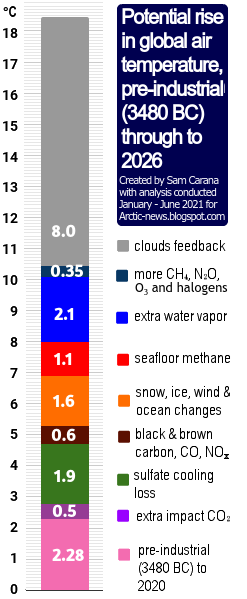
[ from the Extinction page ]
The image on the right is a later version of an image dating back to 2016 that warns about the importance of taking into account a potentially huge rise soon. Disappearance of Antarctic sea ice would be a horrendous climate disaster, increasing the likelihood of a subsequent Arctic Blue Ocean Event. The danger is that multiple feedbacks associated with sea ice loss, such as albedo loss, will strongly accelerate the temperature rise, as warned about at Double Blue Ocean Event and the Antarctica page.

Eruptions of methane from the seafloor could, on their own, cause the 1200 ppm CO₂e cloud feedback tipping point to be crossed, which in turn can cause global temperatures to rise by 8°C, as discussed in this earlier post.

Temperatures look set to rise further due to the falling away of sulfate aerosols, while there could be a additional temperature rises due to releases of other aerosols that have a net warming impact, such as black and brown carbon, which can increase dramatically due to more wood burning and forest fires taking place as industrial activity collapses.

Pursuing efforts?

Most nations have meanwhile ratified the Paris Agreement, which means that politicians are legally obliged to adhere to the Paris Agreement thresholds. However, after more than a decade of pursuing efforts, little or no progress appears to have been made.

The temperature rise is clearly accelerating and denying such acceleration is yet another sick trick in the books of the politicians who control the IPCC, next to using an inappropriate base (instead of pre-industrial), ignoring parts of the current and future temperature rise, and inappropriately using linear trends, even when polynomials obviously work better.

Conclusion

A decade ago, the post concluded as follows: the situation is dire and calls for comprehensive and effective action as described in the Climate Plan. This applies even more today. The situation is dire and unacceptably dangerous, and the precautionary principle necessitates the danger to be acknowledged, while facilitating rapid, comprehensive and effective action to reduce the damage and to improve the outlook, where needed in combination with a Climate Emergency Declaration, as described in posts such as in this 2022 post and this 2025 post, and as discussed in the Climate Plan group. For an update of the Climate Plan, see the Climate Plan by Sam Carana. 

Links

• Pursuing efforts? (2016)
the image at the top is discussed on facebook at

• NASA GISS Surface Temperature Analysis (GISTEMP)

• A recent doubling of global warming rate signals a 1.5 °C breach by 2028 - by Qinjian Jin et al. (2026) 

• Global Warming Rate Has Recently Doubled Meaning We Pass 1.5C By 2028 and 2.0C by as Early as 2038 - video by Paul Beckwith
discussed on facebook at

• Global warming in the pipeline - by James Hansen et al. (2023)

• Pre-industrial

• Paris Agreement (2015)


• When Will We Die? (2019)

• Extinction (2016)

• Transforming Society (2022)

Friday, January 19, 2024

Potential temperature trends

[ click on images to enlarge ]

The above image shows potential temperature trends. Four of the trends are global ones and one trend is based on Arctic (64°North-90°North) data:

  • The red line is a polynomial trend based on 15 years of Arctic data (2009-2023).
  • The green line is a linear trend based on 1880-2023 global data.
  • The yellow line is a linear trend based on 2009-2023 global data.
  • The light blue line is a 10-year moving average (trailing), based on global data.
  • The dark blue line is a polynomial trend, based on 2015-2023 global data, showing global temperatures catching up with the Arctic rise in temperature.

Note that the above image uses annual anomalies from 1951-1980. Recent posts show that, when adjustments are made for an earlier base, for ocean air temperatures and for higher polar anomalies, the 2023 anomaly could be as high as 2.5°C from pre-industrial and when using monthly data, the anomaly could be as high as 2.73°C from pre-industrial. 

Temperature rise hits Arctic most strongly 

Due to feedbacks such as sea ice loss, the temperature rise is felt most strongly at higher latitudes North, as illustrated by the three images below, again using a 1951-1980 baseline.

The image below shows the December 2023 temperature anomaly. 

The image below shows the 2023 temperature anomaly. 

The image below shows how the temperature rise has unfolded from 2000.  

[ Arctic Ocean hit most strongly by temperature rise ]

Over the next few years, the temperature rise in the Arctic could accelerate even more strongly as a result of crossing of two tipping points, i.e. the Latent Heat Tipping Point and the Seafloor Methane Tipping Point, as illustrated by the image below, from an earlier post.

[ increasing ocean heat ]
Note again that annual data are used in the above image. An earlier analysis using monthly data shows that the seafloor methane tipping point was reached in August 2023.

Arctic sea ice extent

Arctic sea ice extent in 2024 was larger than many expected. One of the reasons for this is that Greenland ice has been melting faster than previously thought, as pointed out by a recent study that also includes retreat of glaciers that already lie mostly below sea level. More melting of ice on Greenland has resulted in a larger south-bound flow of icebergs and meltwater, contributing to cooling of the North Atlantic sea surface and slowing down of the Atlantic meridional overturning circulation (AMOC), and in turn contributing to suppress temperatures in the Arctic. As a result, loss of Arctic sea ice extent has been less than would otherwise have been the case. Yet, the temperature rise may soon overwhelm this suppression.

Cold freshwater lid at surface of North Atlantic

[ ocean stratification, from earlier post ]

Slowing down of AMOC and cooling due to heavier melting of Greenland's ice is causing less ocean heat to reach the Arctic Ocean, while a huge amount of ocean heat is accumulating in the North Atlantic, as it did in 2023. A large part of this heat in the North Atlantic can also be present underneath the sea surface.

These developments occur at the same time as ocean stratification increases (see above image) as temperatures rise, as more freshwater enters the ocean as a result of more meltwater and of runoff from land and from rivers, and as more evaporation takes place and more rain falls further down the path of the Gulf Stream, all of which can contribute to formation and growth of a cold, freshwater lid at the surface of the North Atlantic.

[ cold freshwater lid on North Atlantic ]

Furthermore, storms can get stronger as temperatures rise and as changes take place to the Jet Stream. Strong wind can temporarily speed up currents that carry huge amounts of ocean heat with them toward the Arctic Ocean, as discussed in earlier posts such as this one. Much of the ocean heat in the North Atlantic can therefore be pushed abruptly underneath this freshwater lid and flow into the Arctic Ocean.

The danger is that huge amounts of ocean heat can abruptly get pushed into the Arctic Ocean and that the influx of ocean heat will destabilize hydrates contained in sediments at the seafloor of the Arctic Ocean, resulting in eruptions of huge amounts of methane.

[ click on images to enlarge ]

This danger is further illustrated by the above compilation image, showing forecasts for January 27, 2024 of:
(1) surface wind and temperature (-3.6°C or 25.4°F at the North Pole)
(2) surface wind
(3) wind at 700 hPa
(4) wind at 250 hPa (Jet Stream) and
(5) ocean currents at surface and wave height.

The image below shows that temperatures are forecast to be above freezing near the North Pole on January 26, 2024 20:00 UTC (downloaded January 26, 2024 06:00 UTC). 


Ominously, the North Atlantic sea surface was much hotter in early 2024 than it was in early 2023.


And ominously, the daily sea surface temperature reached a record high on January 31, 2024, when the daily sea surface temperature reached 21.10°C, higher than the peak of 21.09°C reached in August 2023 and much higher than the 20.99°C peak reached in March 2016.


As latent heat buffer shrinks, Arctic sea ice could melt away quickly

As illustrated by the image below, sea ice was very thin near the North Pole on January 24, 2024, indicating there is very little left of the latent heat buffer constituted by the sea ice to consume incoming heat. 
And even more ominously, Arctic sea ice thickness declined dramatically in a few days time, as indicated by the compilation image below, with images from the University of Bremen. 


For the time of year, Arctic sea ice extent is currently still extensive, compared to earlier years, which is a reflection of more water vapor in the atmosphere and more precipitation. While sea ice extent is relatively large, Arctic sea ice volume now is among the lowest of all years on record for the time of year, as illustrated by the image below. Volume = extent x thickness, so low volume and relatively large extent means that sea ice is very thin. 
As more sunlight starts reaching the Northern Hemisphere, in line with seasonal changes, Arctic sea ice extent can be affected dramatically and abruptly, as illustrated by the image below.

Furthermore, much of the thicker sea ice is located off the east coast of Greenland, as illustrated by the image below. This means that this sea ice is likely to melt away quickly as temperatures rise in line with seasonal changes.
Without the buffer constituted by thicker sea ice, such an influx of ocean heat could destabilize hydrates contained in sediments at the seafloor of the Arctic Ocean, resulting in eruptions of huge amounts of methane. 
[ The buffer is gone - Latent Heat Tipping Point crossed ]

Given methane's very high immediate global warming potential (GWP), this could push up temperatures dramatically and rapidly. 

[ potential methane rise, from earlier post ]

[ from the Extinction page ]
The above image shows a polynomial trend added to NOAA globally averaged marine surface monthly mean methane data from April 2018 to November 2022, pointing at 1200 ppm CO₂e (carbon dioxide equivalent) getting crossed in 2027.

A rise in methane concentrations alone may suffice to cause the Clouds Tipping Point, at 1200 ppm CO₂e, to get crossed. The resulting clouds feedback could on its own cause the temperature to rise by a further 8°C. 

When further forcing is taken into account, crossing of the Clouds Tipping Point could occur even earlier than in 2027.

The image on the right illustrates how a huge temperature could unfold and reach more than 18°C above pre-industrial by 2026.

With such a rise, the temperature is likely to keep rising further, with further water vapor accumulating in the atmosphere once the water vapor tipping point gets crossed, as discussed in an earlier post and at Could Earth go the same way as Venus? 

As a rather sobering footnote, humans will likely go extinct with a 3°C rise and most life on Earth will disappear with a 5°C rise, as illustrated by the image below, from an earlier post.
[ from earlier post ]

Climate Emergency Declaration

The situation is dire and the precautionary principle calls for rapid, comprehensive and effective action to reduce the damage and to improve the situation, as described in this 2022 post, where needed in combination with a Climate Emergency Declaration, as discussed at this group.


Links

• NASA - Goddard Institute for Space Studies (GISS) Surface Temperature Analysis
https://data.giss.nasa.gov/gistemp

• Ubiquitous acceleration in Greenland Ice Sheet calving from 1985 to 2022 - by Char Greene et al. https://www.nature.com/articles/s41586-023-06863-2
discussed at facebook at: 
https://www.facebook.com/groups/arcticnews/posts/10161223121909679

• Danish Meteorological Institute - Arctic sea ice volume and thickness
https://ocean.dmi.dk/arctic/icethickness/thk.uk.php

• Cold freshwater lid on North Atlantic
https://arctic-news.blogspot.com/p/cold-freshwater-lid-on-north-atlantic.html

• Latent Heat
https://arctic-news.blogspot.com/p/latent-heat.html

• Pre-industrial
https://arctic-news.blogspot.com/p/pre-industrial.html

• Could Earth go the same way as Venus?

Monday, November 16, 2020

Accelerated global warming and stadial cooling events: IPCC oversights regarding future climate trends

 by Andrew Glikson

The linear nature of global warming projections by the IPCC (2014) Assessment Report (AR5) (Figure 1) appears to take little account of stadial cooling events, such as have followed peak temperature rises in previous interglacial stages. The linear trends appear to take only limited account of amplifying positive feedback effects of the warming from land and ocean. A number of factors cast doubt on IPCC climate change projections to 2100 AD and 2300 AD, including:
Figure 1 (a) IPCC average surface temperature change to 2100 relative to 1986-2005 IPCC AR5;
(b) IPCC average surface temperature change to 2300 relative to 1986-2005 IPCC AR5

However, global temperature measurements for 2015-2020 indicate accelerated warming due to both the greenhouse effect reinforced by a solar radiation maximum (Hansen and Sato 2020) (Figure 2).

Figure 2. Accelerated Global Warming reinforced by both greenhouse 
gases and a solar maximum Hansen and Sato, 2020

The weakening of the northern Jet stream, due to polar warming and thus reduced longitudinal temperature contrasts, allows penetration of warm air masses into the polar region and consequent fires (Figure 3). The clash between tropical and polar air and water masses (Figure 3A) leads to regional storminess and contrasting climate change trajectories in different parts of the Earth, in particular along land-ocean boundaries and island chains. 

The weakening of the jet stream and migration of climate zones constitute manifestations of an evolving Earth’s energy imbalance¹, namely a decrease in reflection of solar radiation from Earth to space and thereby global warming. Earth retained 0.6 Watt/m² during 2005-2010 and 0.87 Watt/m² during 2010-2020 (Hansen and Sato 2020), primarily due to a rise in greenhouse gases but also due to a solar radiation peak. During 2015-2020 global warming rates exceeded the 1970-2015 warming rate of 0.18°C/per decade, a deviation greater than climate variability. Hansen and Sato (2020) conclude the accelerated warming is caused by an increasing global climate forcing, specifically by the role of atmospheric aerosols.

Figure 3 A. Undulating and weakening jet stream and the polar vortex and penetration
of warm air, inducing Arctic warming and fires.     B. Satellite images of Wildfires
ravaging parts of the Arctic
, with areas of Siberia, Alaska, Greenland and Canada
engulfed in flames and smoke. While wildfires are common at this time of year, record-
breaking summer temperatures and strong winds have made 2020 fires particularly bad.

Bronselaer et al., 2018 modelled a meltwater-induced cooling of the southern hemisphere toward the end 21st century by as low as -1.5°C (Figure 4A). Hansen et al. 2016 estimated the time frame of 21st century stadial cooling event as dependent on the rates of ice melt (Figure 4B), reaching near global extent toward the end of the century (Figure 4C).

Figure 4 A. 2080–2100 meltwater-induced sea-air temperature anomalies relative to
the standard RCP8.5 ensemble (Bronselaer et al., 2018). Hatching indicates where the
anomalies are not significant at the 95% level;  B. Negative temperature anomalies
through the 21st-22nd centuries signifying stadial cooling intervals (Hansen et al., 2016);
C. A model of Global warming for 2096, where cold ice melt water occupies large parts
of the North Atlantic and circum-Antarctica, raises sea level by about 5 meters and
decreases global temperature by -0.33°C (Hansen et al., 2016).

With the concentration of greenhouse gases rising by approximately 47% during the last century and a half, faster than almost any observed rise in the Cenozoic geological record, the term “climate change” refers to an extreme shift in state of the atmosphere-ocean system. The greenhouse gas rise and temperature rise rates are faster than those of the K-T mass extinction, the Paleocene-Eocene extinction and the last glacial termination.

The consequences for future climate change trends include:
  • Further expansion of the tropical climate zones and a polar-ward shift of intermediate climate zones, leading to encroachment of subtropical deserts over fertile Mediterranean zones. 
  • Spates of regional to continent-scale fires, including in Brazil, Siberia, California, around the Mediterranean, Australia.
  • A weakened undulating jet stream (Figure 3) allowing penetration of and clashes between warm and cold air and water masses, with ensuing storms. 
  • In Australia the prolonged drought, low vegetation moisture, high temperatures and warm winds emanating from the northern Indian Ocean and from the inland, rendering large parts of the continent tinder dry and creating severe fire weather subject to ignition by lightning.
  • The delayed melting of the large ice sheets due to hysteresis², would be followed by sea level rise to Pliocene levels, ~25 meters above pre-industrial levels, once sea level reaches equilibrium with temperature of 2 to 3 degrees Celsius or higher, changing the geography of the continents.
It would follow from these considerations that succeeding periods of peak temperatures, extensive melting of the ice sheets, flow of ice melt into the oceans and thereby stadial cooling would lead to clashes between tropical fronts and cooling masses of air, producing storminess, in particular along continental margins and island chains. The modelled time frame of these developments (Figure 4B) may be cyclical, or may extend further in time and place as long as the ice sheets continue to breakdown.


¹ Earth's energy imbalance is the difference between the amount of solar energy
absorbed 
by Earth and the amount of energy the planet radiates to space as heat.
If the imbalance is 
positive, more energy coming in than going out, we can expect
Earth to become warmer in t
he future — but cooler if the imbalance is negative.
² Hysteresis is the dependence of the state of a system on its history. For example the 
melting of an ice sheet may occur slowly depending on its previous state.

Andrew Glikson

Dr Andrew Glikson
Earth and Paleo-climate scientist
ANU Climate Science Institute
ANU Planetary Science Institute
Canberra, Australia


Books:
The Asteroid Impact Connection of Planetary Evolution
http://www.springer.com/gp/book/9789400763272
The Archaean: Geological and Geochemical Windows into the Early Earth
http://www.springer.com/gp/book/9783319079073
Climate, Fire and Human Evolution: The Deep Time Dimensions of the Anthropocene
http://www.springer.com/gp/book/9783319225111
The Plutocene: Blueprints for a Post-Anthropocene Greenhouse Earth
http://www.springer.com/gp/book/9783319572369
Evolution of the Atmosphere, Fire and the Anthropocene Climate Event Horizon
http://www.springer.com/gp/book/9789400773318
From Stars to Brains: Milestones in the Planetary Evolution of Life and Intelligence
https://www.springer.com/us/book/9783030106027
Asteroids Impacts, Crustal Evolution and Related Mineral Systems with Special Reference to Australia
http://www.springer.com/us/book/9783319745442


Friday, October 26, 2012

Big changes in Arctic within years

Above interactive graphic illustrates the decline of the annual sea ice minimum volume in the Arctic over the years.

What trend can best be fitted to these data? Below, I've added a trendline that I believe best fits the data, but I encourage others to come up with better trends.


The trend points at 2014 as the year when Arctic sea ice will first reach zero volume for some time during that year. As discussed in the earlier post Getting the Picture, the Arctic Ocean looks set to be ice-free for a period of at least three months in 2015 (August, September and October), and for a period of at least 6 months from the year 2020 (June through to November).

Natural variability and strong feedbacks may speed things up further. Decline of sea ice in 2012 was such that we can expect a very low volume in December 2012, which could lead to inclusion of December in the period projected to be ice-free from 2020. That would make the ice-free period seven month long, i.e. well over half a year.

The image below shows the three areas where albedo change will be felt most in the Arctic, i.e. sea ice loss, decline of albedo in Greenland and more early and extensive retreat of snow and ice cover in other areas in the Arctic.


Related

- Getting the Picture
arctic-news.blogspot.com/2012/08/getting-the-picture.html

- Albedo change in the Arctic
arctic-news.blogspot.com/2012/07/albedo-change-in-arctic.html

- Greenland is melting at incredible rate
arctic-news.blogspot.com/2012/07/greenland-is-melting-at-incredible-rate.html

- Albedo change in the Arctic threatens to cause runaway global warming