Friday, February 12, 2021

The extreme rate of global warming: IPCC Oversights of future climate trends

by Andrew Glikson

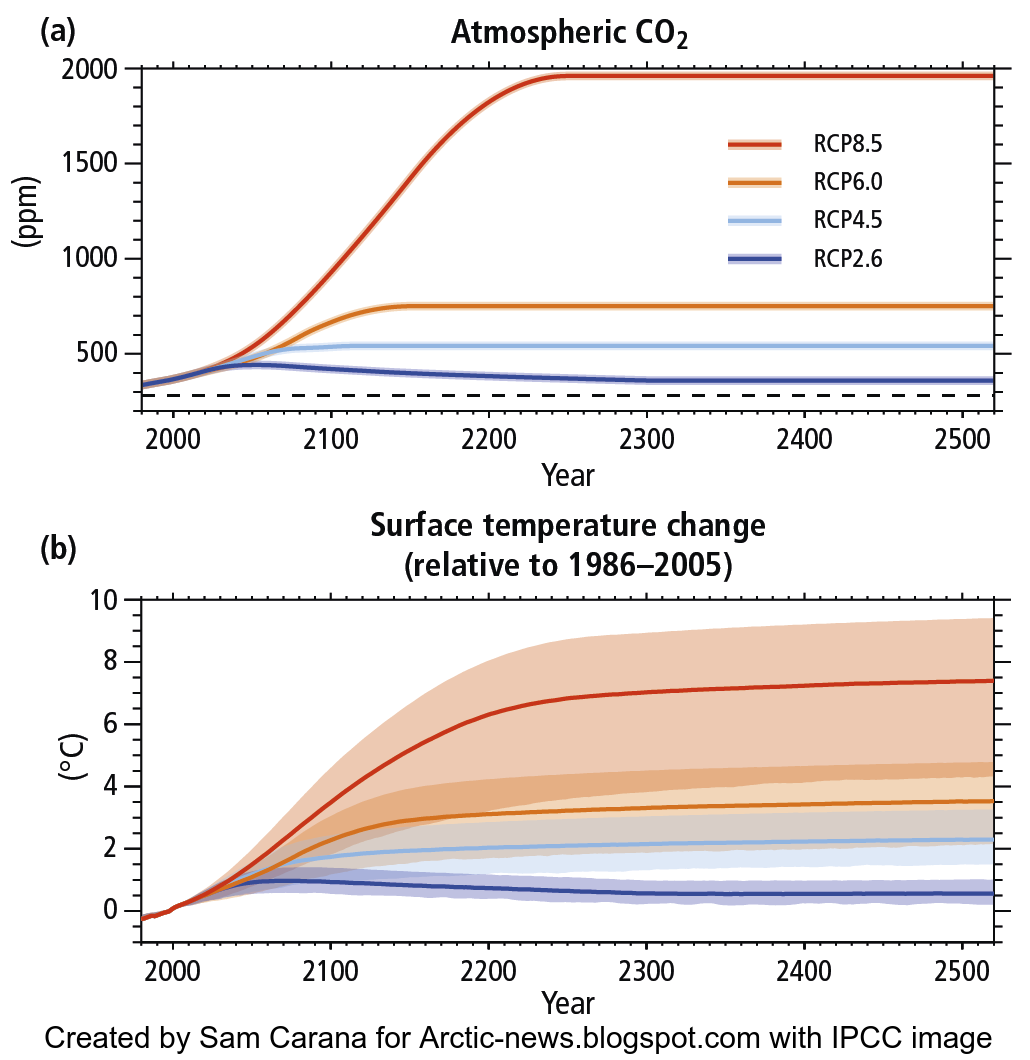
Intergovernmental Panel on Climate Change (IPCC) reports and comprehensive summaries of the peer-reviewed literature raise questions regarding the assumptions inherent in computer modelling of future climate changes, including the supposed linearity of future global temperature trends (Figure 1).

Figure 1. Global mean surface temperature increase as a function of cumulative total global carbon dioxide (CO2) emissions from various lines of evidence. IPCC

Computer modelling does not necessarily capture the sensitivity, complexity and feedbacks of the atmosphere-ocean-land system as observed from paleoclimate studies. Underlying published IPCC computer models appears to be an assumption of mostly gradual or linear responses of the atmosphere to compositional variations. This overlooks self-amplifying effects and transient reversals associated with melting of the ice sheets. 

Leading paleoclimate scientists have issued warnings regarding the high sensitivity of the atmosphere in response to extreme forcing, such as near-doubling of greenhouse gas concentrations: According to Wallace Broecker, “The paleoclimate record shouts out to us that, far from being self-stabilizing, the Earth's climate system is an ornery beast which overreacts to even small nudges, and humans have already given the climate a substantial nudge”. As stated by James Zachos, “The Paleocene hot spell should serve as a reminder of the unpredictable nature of climate”.

Holocene examples are abrupt stadial cooling events which followed peak warming episodes which trigger a flow of large volumes of ice melt water into the oceans, inducing stadial events. Stadial events can occur within very short time, as are the Younger dryas stadial (12.9-11.7 kyr) (Steffensen et al. 2008) (Figure 2) and the 8.2 kyr Laurentian cooling episode,

Despite the high rates of warming such stadial cooling intervals do not appear to be shown in IPCC models (Figure 1).

Figure 2. The younger dryas stadial cooling (Steffensen et al., 2008). Note the abrupt freeze and thaw boundaries of ~3 years and ~1 year.

Comparisons with paleoclimate warming rates follow: The CO₂ rise interval for the K-T impact is estimated to range from instantaneous to a few 10³ years or a few 10⁴ years (Beerling et al, 2002), or near-instantaneous (Figure 3A). An approximate CO₂ growth range of ~0.114 ppm/year applies to the Paleocene-Eocene Thermal Maximum (PETM) (Figure 3B) and ~0.0116 ppm/year to the Last Glacial Termination (LGT) during 17-11 kyr ago (Figure 3C). Thus the current warming rate of 2 to 3 ppm/year is about or more than 200 times the LGT rate (LGT: 17-11 kyr; ~0.0116 ppm/yr) and 20-30 times faster than the Paleocene-Eocene Thermal Maximum (PETM) rate of ~0.114 ppm/year.

Therefore the term “climate change” for the extreme warming reaching +1.5°C over the continents and more than +3°C over the Arctic over a period of less than 100 years, requires reconsideration.

However, comparisons between the PETM and current global warming may be misleading since, by distinction from the current existence of large ice sheets on Earth, no ice was present about 55 million years ago.

Figure 3. (A) Reconstructed atmospheric CO₂ variations during the Late Cretaceous–early Tertiary, based on -
Stomata indices of fossil leaf cuticles calibrated using inverse regression and stomatal ratios (Beerling et al. 2002);
(B) Simulated atmospheric CO₂ at and after the Palaeocene-Eocene boundary (after Zeebe et al., 2009);
(C) Global CO₂ and temperature during the last glacial termination (After Shakun et al., 2012) (LGM - Last Glacial Maximum; OD – Older dryas; BA - Bølling–Alerød; YD - Younger dryas)

Observed climate complexities leading to the disturbance of linear temperature variations include:
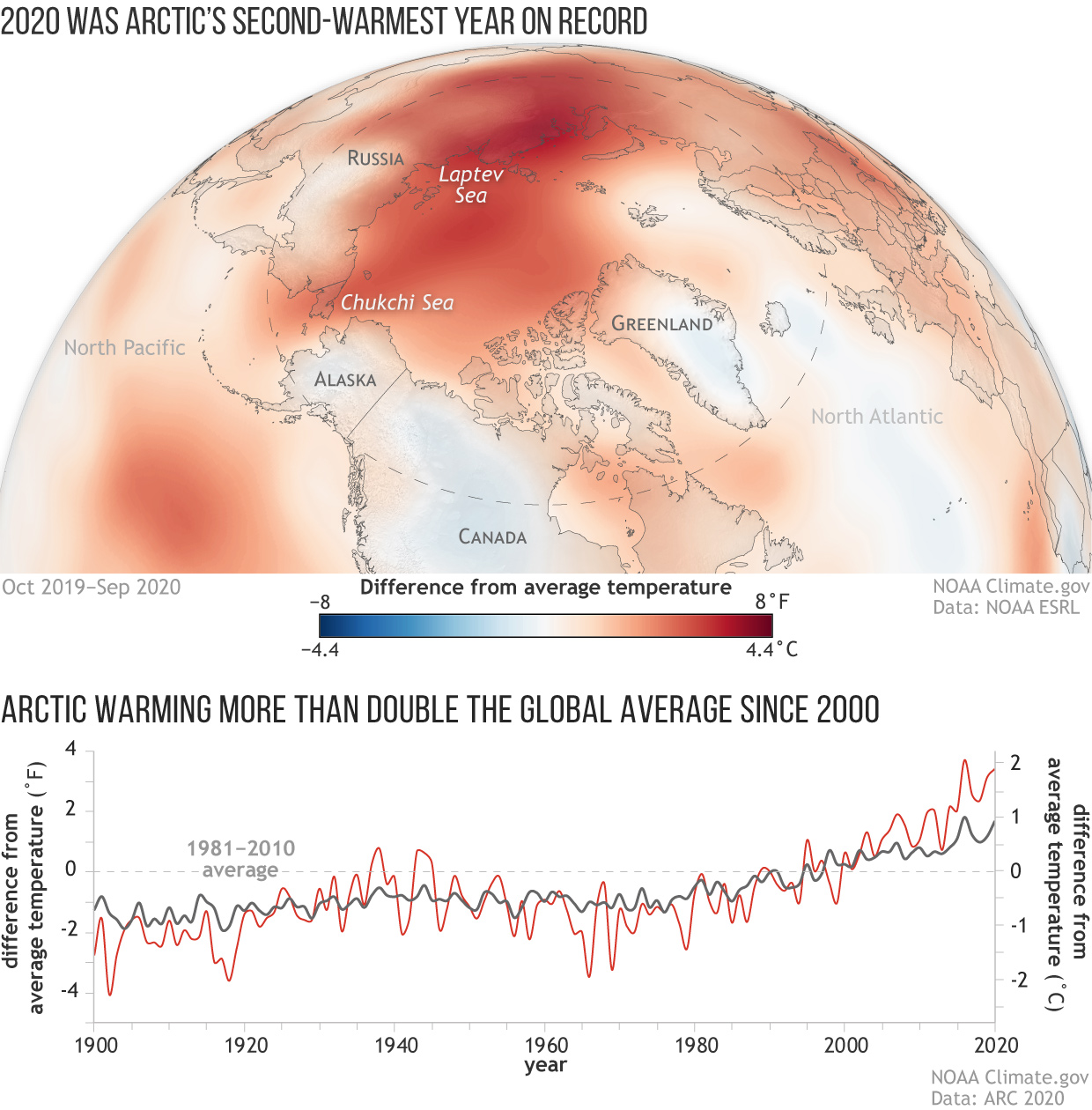
  1. The weakening of climate zone boundaries, such as the circum-Arctic jet stream, allowing cold air and water masses to shift from polar to mid-latitude zones and tropical air masses to penetrate polar zones (Figure 4), induce collisions between air masses of contrasted temperatures and storminess, with major effects on continental margins and island chains.

  2. Amplifying feedbacks, including release of carbon from warming oceans due to reduced CO₂ solubility and therefore reduced intake from the atmosphere, release of methane from permafrost and from marine sediments, desiccated vegetation and extensive bush fires release of CO₂.

  3. The flow of cold ice melt water into the oceans from melting ice sheets—Greenland (Rahmstorf et al., 2015) and Antarctica (Bonselaer et al., 2018)—ensuing in stadial cooling effects, such as the Younger dryas and following peak interglacial phases during the last 800,000 years (Cortese et al., 2007; Glikson, 2019).
Figure 4. Weakening and undulation of the jet stream, shifts of climate zones and penetration of air masses across the weakened climate boundary. NOAA.

In the shorter term such international targets as “zero emissions by 2050” apparently do not include the export of petroleum, coal and gas, thus allowing nations to circumvent domestic emission limits. Australia, the fifth biggest miner and third biggest exporter of fossil fuels, is responsible for about 5% of global greenhouse gas emissions.

At present the total CO₂+CH₄+N₂O level (mixing ratio) is near 500 ppm CO₂-equivalent (Figure 5). From the current atmospheric CO₂ level of above ~415 ppm, at the rise rate of 2 - 3 ppm/year, by 2050 the global CO₂ level would reach about 500 ppm and the CO₂-equivalent near 600 ppm, raising mean temperatures to near-2°C above preindustrial level, enhancing further breakdown of the large ice sheets and a further rise of sea levels.

Figure 5. Evolution of the CO₂+CH₄+N₂O level (mixing ratio)


Andrew Glikson

Dr Andrew Glikson
Earth and Paleo-climate scientist
ANU Climate Science Institute
ANU Planetary Science Institute
Canberra, Australia


Books:
The Asteroid Impact Connection of Planetary Evolution
http://www.springer.com/gp/book/9789400763272
The Archaean: Geological and Geochemical Windows into the Early Earth
http://www.springer.com/gp/book/9783319079073
Climate, Fire and Human Evolution: The Deep Time Dimensions of the Anthropocene
http://www.springer.com/gp/book/9783319225111
The Plutocene: Blueprints for a Post-Anthropocene Greenhouse Earth
http://www.springer.com/gp/book/9783319572369
Evolution of the Atmosphere, Fire and the Anthropocene Climate Event Horizon
http://www.springer.com/gp/book/9789400773318
From Stars to Brains: Milestones in the Planetary Evolution of Life and Intelligence
https://www.springer.com/us/book/9783030106027
Asteroids Impacts, Crustal Evolution and Related Mineral Systems with Special Reference to Australia
http://www.springer.com/us/book/9783319745442


Wednesday, February 3, 2021

More Extreme Weather

As temperatures rise, the weather is getting more extreme. Around the globe, extreme weather events are striking with ever greater frequency and intensity. 

In 2020, in the U.S. alone, a record number of 22 climate and weather disasters took place that each caused damage of more than 1 billion dollar, while jointly causing the deaths of 262 people. 

Rising temperatures cause stronger storms, droughts, heatwaves and forest fires. Rising temperatures are also behind the cold weather that is currently hitting large parts of North America. Two mechanisms that, by distorting the Jet Stream, are contributing to more extreme weather are described below. 

Distortion of the Jet Streams - two mechanisms

The Jet Streams used to circumnavigate the globe in narrow bands. World climate zones used to be kept well apart by stable Jet Streams. 

On the Northern Hemisphere, the coldest point used to be the North Pole, so wind used to flow from the tropics to the North Pole, while the wind was moved to the side due to Earth's turning. 

Polar Jet Stream and Subtropical Jet Stream - NOAA image
This resulted in two Jet Streams forming, circum-navigating the globe in relatively narrow and straight bands, i.e. the Polar Jet Stream at 60°N and the Subtropical Jet Stream at about 30°N. 
 
Polar Jet Stream (blue) and Subtropical
Jet Stream (red) - NOAA image
First mechanism distorting the Jet Stream

The first mechanism distorting the Jet Stream is that, as the Arctic gets hit much harder by temperature rises, the difference in temperature decreases between the North Pole and the Equator.

This slows down the speed at which wind travels from the Tropics to the North Pole, in turn making the Jet Stream more wavy, just like a slow-moving river over flat land will take a winding route and meander.

For years, Jennifer Francis et al. warned that this will cause more extreme weather in mid latitudes. Arctic-News described Deformation of the Jet Stream as Opening the Doorways to Doom, i.e. one of the feedbacks (#10) of accelerated Arctic warming.

Second mechanism distorting the Jet Stream

Due to the rapid temperature rise of the Arctic Ocean, the North Pole is increasingly not the coldest place on the Northern Hemisphere.

Instead, the air over Greenland, North Canada and Siberia is increasingly more cold than before, and can be much colder than the North Pole, as illustrated by the ClimateReanalyzer image on the right.

This creates temperature and pressure conditions over the East Pacific and over North America that make the Jet Stream branch out.

On the next image on the right, the Jet Stream can be seen running over the West Pacific at speeds as high as 387 km/h or 241 mph (green circle) and moving within a narrow and straight band.

The Jet Stream is then confronted with much different conditions over North America that make the Jet Stream branch out widely (white arrows), with one branch moving north and going circular over the Arctic Ocean, while at the other end a branch can be seen dipping below the Equator.

As a result of these two distortion mechanisms, cold air that used to stay contained over the North Pole, can descend more easily over Siberia and North America, causing more extreme weather, while also taking away opportunities for the sea ice to build up to the strength and depth than it used to have. 

The combination image below shows forecasts for February 6, 2021.


On the above combination image, the left panel shows that, not far apart from each other and at the same time, temperature anomalies over North America are forecast to approach the top end and the bottom end of the scale. The right panel shows that temperatures over North America and Siberia are forecast to be much lower than over the Arctic Ocean.

As the temperature difference between land and ocean gets stronger on the Northern Hemisphere in Winter, the transfer of water vapor and heat to the atmosphere increases (#25 on the feedbacks page, image right). Storms and clouds forming over the North Atlantic trap heat and move much heat toward the North Pole.
 
Formation of clouds can be further facilitated by aerosols (feedback #9). A recent study looks at how melting sea ice can cause more release of iodine into the atmosphere, seeding the growth of new clouds that trap longwave radiation that would otherwise go into space.

The combination image below shows in the left panel how a branch of the Jet Stream is forecast to be moving over the North Pole at speeds as high as 107 km/h or 67 mph on February 16, 2021. Hours later that day, as the globe in the right panel shows, the surface temperature on the North Pole is forecast to be -18°C, i.e. warmer than the white-blue color (about -20°C) that covers most of North America.


As the globe in the left panel of the combination image below shows, temperature anomalies in Texas were approaching the bottom end of the scale on February 15, 2021, i.e. -32°C or -57.6°F (below 1979-2000), while the globe in the right panel shows that on February 16, 2021, temperature anomalies in between Greenland and the North Pole were forecast to approach the top end of the scale, i.e. 32°C or 57.6°F (above 1979-2000). 


Above freezing at North Pole?

As the combination image below shows, the temperature at the North Pole is forecast to be 0°C or 32°F, panel right, on February 22, 2021, 18:00 UTC, while temperature anomalies at the North Pole are forecast to be at the top end of the scale, i.e. 32°C or 57.6°F above 1979-2000. 


The light-blue color over the North Atlantic on the globe on the left is a cold anomaly resulting from cold air moving from North America over the Atlantic Ocean (forecast initiated Feb.15, 2021, 18:00 UTC).

Ominously, sea ice is breaking up north of Greenland. 


And ominously, the N20 satellite recorded methane levels as high as 2835 ppb at 399.1 mb on the afternoon of February 17, 2021.


Conclusion

The situation is dire and calls for immediate, comprehensive and effective action as described in the Climate Plan.


Links

• 2020: Hottest Year On Record
https://arctic-news.blogspot.com/2021/01/2020-hottest-year-on-record.html

• NOAA - U.S. Billion-Dollar Weather and Climate Disasters: Overview
https://www.ncdc.noaa.gov/billions/overview

• Climate Reanalyzer
https://climatereanalyzer.org

• Nullschool

• Feedbacks in the Arctic

• Evidence linking Arctic amplification to extreme weather in mid‐latitudes - by Jennifer Francis et al. 

• Opening the Doorways to Doom (feedback #14)


Thursday, January 28, 2021

What Carbon Budget?


Orbital changes are responsible for the Milankovitch cycles that make Earth move in and out of periods of glaciation, or Ice Ages. In line with these cycles, July insolation has slowly decreased over the last 12,000 years. While insolation was at a peak some 12,000 years ago, temperatures rose only slowly at first, as the ice receded that was formed during the most recent Ice Age.

Some previous temperature reconstructions did suggest that a peak on temperature was reached around 6,000 to 7,000 years ago, followed by a decrease in temperature that continued until the industrial age. However, Samantha Bova and colleagues found that most of the records used in such reconstructions represented seasonal temperatures rather than annual ones.

They developed a method of evaluating individual records for seasonal bias and after adjusting for this, they found that the mean annual sea surface temperature has been rising steadily for the past 12,000 years, due to retreating ice sheets during the period from 12,000 to 6,500 years ago and, more recently, due to the increase in greenhouse gas emissions.

Paris Agreement

The Paris Agreement calls for a global average temperature well below 2°C above pre-industrial levels, with efforts taken to ensure that the temperature doesn't exceed 1.5°C above pre-industrial levels.

So, what are pre-industrial levels? The 'pre-' in pre-industrial means before, suggesting that pre-industrial levels refers to levels as they were in times before the Industrial Revolution started.

While emission of greenhouse gases did rise strongly since the start of the Industrial Revolution, the rise in emission of greenhouse gases by people had already started some 7,000 years ago with the rise in modern agriculture and associated deforestation. As this new study shows, the temperature has risen steadily since.

A recent post confirms earlier warnings that the temperature may already have risen by more than 2°C, and it looks even more that way when moving the baseline back 7,000 years. Moreover, this recent post again warns that the temperature rise is accelerating as tipping points are getting crossed, feedbacks are growing stronger and further heating elements are kicking, all interacting in non-linear ways to speed up the temperature rise.

So, where are those efforts that politicians pledged they would be taking?

What Carbon Budget?

Instead of making a genuine effort, most politicians and mainstream media keep telling people that there was a carbon budget to be divided among polluters, as if people should happily continue to consume the polluting products that are pushed by advertisers, for decades to come.

In reality, however, there is no carbon budget, there is no pollution budget. Instead, there is just a huge pollution debt to be paid and every minute of delay causes exponential growth of this debt and of the prospect of rapid human extinction and ultimately extinction of all life on Earth.


Carbon dioxide levels

[ click on images to enlarge ]
The IPCC image on the right shows CO₂ concentrations (up to 2000 ppm) and, underneath, the temperature rise (relative to 1986-2005) for the various RCPs.

What is RCP2.6? As the IPCC described in AR5, the temperature does not rise above 1.5°C (relative to 1850-1900) under the RCP2.6 scenario, and CO₂ concentrations do not rise above 421 ppm.

It looks like CO₂ concentrations will soon cross this 421 ppm threshold, given that the average daily CO₂ level recorded at Mauna Loa, Hawaii, was 419.12 ppm on February 4, 2021, a record high. The next day, February 5, 2021, the daily level was even higher, 419.45 ppm. The annual peak is typically reached in May, so levels can be expected to rise further over the next few months and cross the 421 ppm threshold soon.
 
Crossing the 421 ppm threshold implies that the RCP2.6 scenario is no longer applicable and that politicians won't be able to honour the pledges made at the Paris Agreement without geoengineering.

How much could temperatures rise? The IPCC image shows that the IPCC at the time when AR5 was written expected the temperature to rise by 3.7°C (with a range of 2.6°C to 4.8°C) under RCP8.5 by 2081–2100 relative to 1986–2005, and to keep rising beyond 2100 and reach 7.4°C and possibly 9.4°C relative to 1986–2005 over time.

The IPCC adds that, by 2100, CO₂ concentrations would reach 936 ppm under RCP 8.5., but when also (next to CO₂ concentrations) including the prescribed concentrations of CH₄ and N₂O, the combined CO₂-equivalent concentrations for RCP8.5 is expected to rise to 1313 ppm by the year 2100.

Meanwhile, a study discussed in an earlier post found that when the 1200 ppm CO₂-e gets crossed, the clouds feedback starts to kick in that can push the temperature up by an additional 8°C.

In line with IPCC AR5 figures, methane's Global Warming Potential (GWP) over a few years is 150.

Since AR5 was published, a study found methane's 100 year GWP to be 14% higher than the IPCC value. When applying an extra 14% to methane's short-term GWP of 150, it rises to 171.

Let's take the above (February 5, 2021) CO₂ level of 419.45 ppm and add the WMO 2019 level of methane of 1877 ppb, which with a short-term GWP of 171 translates into heating equivalent of 320.967 ppm CO₂.

Together, the existing CO₂ and methane add up to 740.417 ppm CO₂e, which is 459.583 ppm CO₂e away from the 1200 ppm CO₂e cloud tipping point.

In other words, a methane burst alone could drive up the methane level in the atmosphere by 2688 ppb, resulting in the cloud feedback tipping point to get crossed and the temperature to rise by an additional 8°C. Alternatively, the 1200 ppm CO₂e tipping point could get crossed due to a combination of warming elements, as depicted in the chart below, from a recent post, which would result in a total rise of 18°C when the cloud feedback is added on top. 


Methane

A reduction in carbon dioxide levels in the atmosphere isn't the only thing that's needed to avoid the worst of the looming temperature rise. There are many further lines of action that need to be implemented urgently, including efforts to reduce methane levels. 

Ominously, high methane levels were recorded by the N20 satellite on the morning of January 20, 2021. The combination image below shows levels as high as 2636 ppb at 695 mb (panel left) and 2806 ppb at 487 mb (panel right).


High methane levels were also recorded on January 30, 2021 pm. The combination image below shows that the SNPP satellite recorded levels as high as 2704 ppb at 487 mb (panel left), while the MetOp-2 satellite recorded levels as high as 2344 ppb at 469 mb (panel right). 


On February 4, 2021 pm, the MetOp-1 satellite recorded methane levels of 3071 ppb at 469 mb, as illustrated by the image in the right.

High peak methane levels are very worrying; what makes it even more threatening is that so much of the Arctic Ocean on above images is showing to be covered by high methane levels. 

This supports fears expressed earlier, such as in this recent post, about methane's present and future role in accelerating the temperature rise. 

Nitrous oxide

The image on the right shows nitrous oxide levels at Barrow, Alaska, over the past few years. 

Clearly, action to avoid nitrous oxide releases is also needed urgently.  

Conclusion

The situation is dire and calls for immediate, comprehensive and effective action as described in the Climate Plan.


Links

• Seasonal origin of the thermal maxima at the Holocene and the last interglacial - by Samantha Bova et al.
https://www.nature.com/articles/s41586-020-03155-x

• Palaeoclimate puzzle explained by seasonal variation
https://www.nature.com/articles/d41586-021-00115-x

• Important Climate Change Mystery Solved by Scientists
https://www.rutgers.edu/news/important-climate-change-mystery-solved-scientists

• Milankovitch (Orbital) Cycles and Their Role in Earth's Climate - by Alan Buis (NASA news, 2020)
https://climate.nasa.gov/news/2948/milankovitch-orbital-cycles-and-their-role-in-earths-climate

• Milankovitch cycles - Wikipedia
https://en.wikipedia.org/wiki/Milankovitch_cycles

• Insolation changes
https://energyeducation.ca/encyclopedia/Insolation
http://www.geo.umass.edu/faculty/bradley/bradley2003x.pdf

• Paris Agreement
https://unfccc.int/process-and-meetings/the-paris-agreement/the-paris-agreement
https://unfccc.int/sites/default/files/english_paris_agreement.pdf

• IPCC AR5 Synthesis Report — Figure 2.8

• IPCC AR5 Report, Summary For Policymakers

• Most Important Message Ever
https://arctic-news.blogspot.com/2019/07/most-important-message-ever.html

• Radiative forcing of carbon dioxide, methane, and nitrous oxide: A significant revision of the methane radiative forcing - by M. Etminan et al. 

• Possible climate transitions from breakup of stratocumulus decks under greenhouse warming - by Tapio Schneider et al.
https://www.nature.com/articles/s41561-019-0310-1

• A World Without Clouds

Thursday, January 21, 2021

The peril of high atmospheric methane levels

by Andrew Glikson

It is hard to think of a more Orwellian expression than that describing the increase in toxic atmospheric methane gas as “gas-led recovery.”

Several of the large mass extinctions of species in the geological past are attributed to an increase in atmospheric methane (CH₄), raising the temperature of the atmosphere and depriving the oceans from oxygen. Nowadays a serious danger to the atmosphere and for the life support systems ensues from the accelerated release of methane from melting Arctic permafrost, leaks from ocean sediments and from bogs, triggered by global warming. As if this was not dangerous enough, now methane is extracted as coal-seam-gas (CSG) by fracking (hydraulic fracturing) of coal and oil shale in the US, Canada, Australia and elsewhere.

Methane-bearing formations, located about 300m-1000m underground, are fracked using a mixture of water, sand, chemicals and explosives injected into the rock at high pressure, triggering significant amounts of methane leaks into the overlying formations and escaping into the atmosphere (Figure 1).

Figure 1. Schematic illustration of coal-seam-gas fracking (R. Morrison, by permission).

CSG is made primarily of about 95-97% methane, which possesses a radiative greenhouse potential close to X80 times that of carbon dioxide (CO₂). The radiative greenhouse effect of 1 kg methane is equivalent to releasing 84 kg of CO₂ and decreases to 20 and 34 times stronger than CO₂ over a 100-year period.

Global methane deposits (Figure 2) and Australian methane-bearing basins (Figure 3) are proliferating. Fugitive emissions from CSG are already enhancing the concentration of atmospheric methane above drill sites and range from 1 to 9 percent during the total life cycle emissions. The venting of methane from underground coal mines in the Hunter region of New South Wales has led to an atmospheric level in the region of 3,000 parts per billion, with methane levels of 2,000 ppb (parts per billion) extending to some 50 km away from the mines. Peak readings in excess of 3000 ppb represent an amalgamation of plumes from 17 sources. The median concentration within this section was 1820 ppb, with a peak reading of 2110 ppb. Compare this with mean methane values at Mouna Loa, Hawaii, of 1884 ppb.

Figure 2. Global gas hydrate potential regions.

Fugitive methane emissions from natural, urban, agricultural, and energy-production landscapes of eastern Australia. The chemical signature of methane released from fracking is found in the atmosphere points to shale gas operations as the source.


Figure 3. Australian basins, oil and gas resources.

The accumulation of many hundreds of billions tons of unoxidized methane-rich organic matter in Arctic permafrost, methane hydrates in shallow Arctic lakes and seas, bogs, and as emanated from cattle and sheep, has already enhanced global methane growth over the last 40 years at rates up to 14 ppb/year (Figure 4).


Figure 4. Growth of atmospheric methane, Mouna Loa, Hawaii,
between 1980-2020 and 2017-2020. NOAA.

The current methane level of 1884 ppb, ~2.5 times the <800 ppb level in 1840AD, indicating a mean growth rate of ~7 ppb/year (Figure 4), is attributable to in part to animal husbandry, permafrost melting, release from marine hydrates and bogs, and in part emissions from shale gas and fracking. as in the United States and Canada.

High levels of methane reduce the amount of oxygen breathed from the air, with health consequences. The toxicity of methane is corroborated in a 2018 study in Pennsylvania showing children born within a mile or two of a gas well were likely to be smaller and less healthy. New York State, Maryland, and Vermont have banned fracking, as have France and Germany.

According to Hansen (2018) reserves of unconventional gas exceed 10,000 GtC (billion tons carbon). Given the scale of methane hydrate deposits around the world (Figure 5), sufficient deposits exist to perpetrate a global mass extinction of species on a geological scale.¹ 

Figure 5. Estimates of methane held in hydrates worldwide. Estimates of the Methane Held in Hydrates Worldwide. Early estimates for marine hydrates (encompassed by the green region), made before hydrate had been recovered in the marine environment, are high because they assume gas hydrates exist in essentially all the world’s oceanic sediments. Subsequent estimates are lower, but remain widely scattered (encompassed by the blue region) because of continued uncertainty in the non-uniform, heterogeneous distribution of organic carbon from which the methane in hydrate is generated, as well as uncertainties in the efficiency with which that methane is produced and then captured in gas hydrate. Nonetheless, marine hydrates are expected to contain one to two orders of magnitude more methane than exists in natural gas reserves worldwide (brown square) (U.S. Energy Information Administration 2010). Continental hydrate mass estimates (encompassed by the pink region) tend to be about 1 per cent of the marine estimates.


¹ For 2.12 billion ton of carbon (GtC) raising atmospheric CO₂ by 1ppm, and assuming about 50% of CO₂ remaining in the atmosphere, future drilling and fracking could in principle raise atmospheric CO₂ level to about or more than 2000 ppm.


Andrew Glikson

Dr Andrew Glikson
Earth and Paleo-climate scientist
ANU Climate Science Institute
ANU Planetary Science Institute
Canberra, Australia


Books:
The Asteroid Impact Connection of Planetary Evolution
http://www.springer.com/gp/book/9789400763272
The Archaean: Geological and Geochemical Windows into the Early Earth
http://www.springer.com/gp/book/9783319079073
Climate, Fire and Human Evolution: The Deep Time Dimensions of the Anthropocene
http://www.springer.com/gp/book/9783319225111
The Plutocene: Blueprints for a Post-Anthropocene Greenhouse Earth
http://www.springer.com/gp/book/9783319572369
Evolution of the Atmosphere, Fire and the Anthropocene Climate Event Horizon
http://www.springer.com/gp/book/9789400773318
From Stars to Brains: Milestones in the Planetary Evolution of Life and Intelligence
https://www.springer.com/us/book/9783030106027
Asteroids Impacts, Crustal Evolution and Related Mineral Systems with Special Reference to Australia
http://www.springer.com/us/book/9783319745442