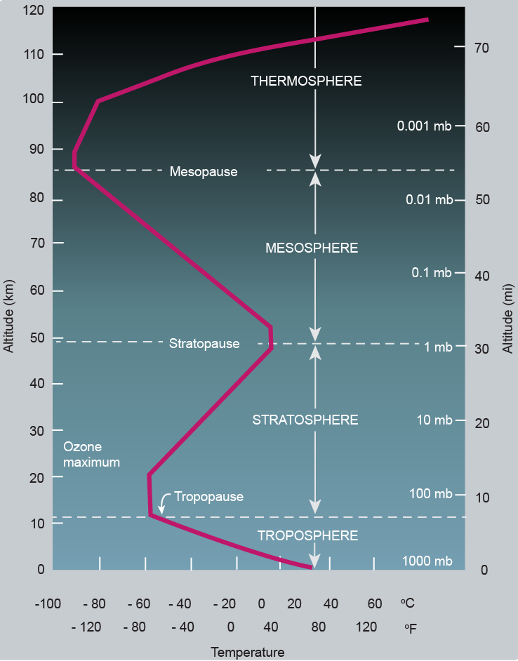
The Atmosphere can be divided into layers. The Troposphere is the layer that is closest to the surface. When rising up in the Atmosphere, the next layer up is the Stratosphere. The next layer up is the Mesosphere and the fourth layer from the bottom is the Thermosphere.
The temperature rises or falls in a different way in each of these layers, as illustrated by the red line in the image CC from archive.nptel.ac.in on the right and the scale on the bottom.
The ozone layer is located in the lower stratosphere at an altitude of 15 to 35 km or 9 to 22 miles above the Earth's surface, with the highest concentrations usually peaking around 25 km. This altitude corresponds with a pressure level of 100 to 10 mb or hPa.
The ozone layer absorbs 97% to 99% of the Sun's medium-frequency ultraviolet light (from about 200 nm to 315 nm wavelength), which otherwise could cause severe damage to life on Earth.
Water vapor rising over Antarctica
The image below shows a temperature anomaly forecast for July 3, 2026. At this time of year very little sunlight is reaching Antarctica, so the temperature over Antarctica can get very low. At the same time, global warming has increased sea surface temperatures and this also keeps air temperatures over water relatively warm. The difference in temperature strengthens wind patterns from the Southern Ocean to Antarctica, which can lead to atmospheric rivers moving toward Antarctica, carrying water vapor and heat from the Southern Ocean to Antarctica.
The red color on the above image indicates high temperature anomalies over Antarctica. The dark blue areas indicate where snow has fallen over the sea ice around Antarctica and over the interior of Antarctica.
As temperatures rise, the water vapor in the air increases. The amount of water vapor that the air can hold rises by 7% for each 1°C temperature rise (Clausius-Clapeyron relation). While much of the water vapor will fall out of the air as precipitation, in the form of rain or snow, some of the water vapor will remain in the air. This extra water vapor increases temperatures, since water vapor is a strong greenhouse gas. The IPCC adds: Water vapor feedback acting alone approximately doubles the warming from what it would be for fixed water vapor. Furthermore, water vapor feedback acts to amplify other feedbacks in models, such as cloud feedback and ice albedo feedback. If cloud feedback is strongly positive, the water vapor feedback can lead to 3.5 times as much warming as would be the case if water vapor concentration were held fixed.
Part of the precipitation will fall over Antarctica in the form of snow, thickening the snow cover there, without returning to the surface of the Southern Ocean. The net result is that the salinity of the Southern Ocean surface increases, facilitating increased melting of Antarctic sea ice, further speeding up the temperature rise, as also discussed in earlier posts such as this one.
The threat is further illustrated by the image below, which shows a forecast of precipitable water standardized anomalies on June 30, 2026.
[ minus 70.2°C near South Pole ]
In the Northern Hemisphere, rising temperatures are narrowing the temperature difference between the Equator and the North Pole, slowing down the wind flow from south to north, resulting in a distorted Jet Stream that goes circular in many areas, and this can increase the severity, intensity, frequency, duration and ubiquity of extreme weather events such as heatwaves and forest fires.
The Jet Stream in the Southern Hemisphere is now very powerful, since the temperature difference is large between the Equator and the South Pole, where temperatures lower than -70°C are recorded, as illustrated by the image on the right.
The situation is further illustrated by the image below, dated July 25, 2026, 09:00 UTC. At a location marked by the green circle, wind at 250 hPa reaches a speed of 321 km/h, while Instantaneous Wind Power Density is 143.1 kW/m².
This can at times cause the Jet Stream to move over parts of Antarctica, enabling warm, moist air to move from the Southern Ocean over Antarctica, which can result in very high temperatures anomalies, as illustrated by the image below that shows a forecast with areas over Antarctica reaching temperature anomalies of about +30°C on July 18, 2026, i.e. winter heatwave conditions in Antarctica.
In the video below, Guy McPherson discussed warming of Antarctica.
Damage to the Ozone Layer
Furthermore, part of the extra water vapor can rise up and moisten the atmosphere up to and above the ozone layer. The combination image below shows relative humidity on June 30, 2026 at 01:00 UTC, with relative humidity reaching up to 100% at surface level (left), up to 100% at 70 mb or hPa (center), and up to 23% at 10 mb or hPa (right).
Increases in stratospheric water vapor are bad news, as they not only speed up global warming but also lead to loss of stratospheric ozone, as Drew Shindell pointed out back in 2001.
It has long been known that deterioration of the ozone shield increases ultraviolet-B irradiation, in turn causing skin cancer.
Research (box right) suggests that, millions of years ago, it could also have led to loss of fertility and consequent extinction in plants and animals.
Water vapor reaching stratospheric altitudes causes ozone depletion, as James Anderson describes in a 2017 paper and discusses in the short 2016 video below.
A recent study led by Yifeng Peng finds that moderate volcanic eruptions and extreme wildfires since 2005 have systematically increased stratospheric water vapor. Both contribute through aerosol-induced tropopause warming; extreme wildfires also reveal an additional self-lofting pathway that transports water vapor into the stratosphere.
Conclusion
The image below shows annual maximum daily precipitation change with a temperature versus 1850-1900 rise of 1.5°C, 2°C, and 4°C, from the IPCC AR6.
The situation looks set to deteriorate further. More water vapor causes more warming, since water vapor is a potent greenhouse gas. As more snow falls over Antarctica, the sea surface of the Southern Ocean increases in salinity, which speeds up melting of sea ice. The extra water vapor and increased melting of sea ice can both strongly accelerate the temperature rise, while water vapor that reaches the stratosphere also causes damage to the ozone layer.
The situation is dire and unacceptably dangerous, and the precautionary principle necessitates the danger to be acknowledged, while facilitating rapid, comprehensive and effective action to reduce the damage and to improve the outlook, where needed in combination with a Climate Emergency Declaration, as described in posts such as in this 2022 post and this 2025 post, and as discussed in the Climate Plan group.
A 5 Gt burst of seafloor methane would nearly double the methane in the atmosphere and could instantly raise CO₂e level to well above 1200 ppm, thus triggering the cloud feedback.
The above image looks into a scenario in which methane concentrations nearly double, due to 5 Gt of methane getting released, instantly increasing CO₂e levels to above 1200 ppm and thus triggering the cloud feedback, as described in the image and as illustrated by the bar on the right in the above image.
Importantly, the clouds tipping point could also be crossed with far less methane getting released. As illustrated by the bar on the left in the above image, levels of further pollutants could increase rapidly while feedbacks strengthen and while sulfate cooling ends abruptly, causing the clouds tipping point to get crossed and resulting in a potential rise of 18.44°C (from pre-industrial) by the end of 2026, as also discussed at the extinction page.
Climate Emergency Declaration
The situation is dire and unacceptably dangerous, and the precautionary principle necessitates rapid, comprehensive and effective action to reduce the damage and to improve the outlook, where needed in combination with a Climate Emergency Declaration, as described in posts such as in this 2022 post and this 2025 post, and as discussed in the Climate Plan group.
Forecast of Wet Bulb Globe Temperature of 35°C or 96°F in south of Texas, U.S.
A temperature of 39°C or 102°F is forecast for a location in the south of Texas, U.S., for June 18, 2026 20 UTC. With a relative humidity of 51%, this translates into a 'feels like' temperature of 52°C or 125°F and a Wet Bulb Globe Temperature of 35°C or 96°F.
Furthermore, as illustrated by the image below, a temperature of 41°C or 105°F is forecast for another location in the south of Texas, U.S., for June 18, 2026 20 UTC. With a relative humidity of 44%, this translates into a 'feels like' temperature of 52°C or 126°F and a Wet Bulb Globe Temperature of 35°C or 96°F.
Wet Bulb Globe Temperature of 36°C or 97°F forecast to hit location in California
The image below shows a temperature of 47°C or 116°F forecast to hit a location in the south of California on July 25, 2026, 21:00 UTC. With a relative humidity of 17%, this translates into a 'feels like' temperature of 48°C or 119°F and a Wet Bulb Globe Temperature of 36°C or 97°F.
Wet-bulb and wet-bulb globe temperature
The wet bulb temperature measures the lowest temperature to which an object can cool down through the evaporation of water, primarily accounting for heat and humidity in the shade.
According to NOAA, the Wet Bulb Globe Temperature (WBGT) is an indicator of heat related stress on the human body in direct sunlight. It takes into account multiple atmospheric variables, including: temperature, humidity, wind speed, sun angle, and cloud cover.
The human body can cool itself by sweating and the stronger the wind, the more one can cool off by sweating. As temperatures and humidity levels keep rising, a threshold can be reached or exceeded where the wind factor no longer matters, in the sense that wind can no longer provide cooling. This physiological limit was long described as a 35°C wet-bulb temperature. i.e. once the wet-bulb temperature reaches this limit, one can no longer lose heat by perspiration, even in strong wind, but instead the human body will start gaining heat from the air beyond a wet-bulb temperature of 35°C.
The image below shows a forecast for July 26, 2026, 21:00 UTC. The image shows a temperature of 122°F (50°C) at a location near Death Valley with a relative humidity of 9% resulting in a wet bulb globe temperature of 95°F (35°C). At the same time, a temperature of 116°F (47°C) with a relative humidity of 20% results in a wet bulb globe temperature of 97°F (36°C) at a location in the south of California.
A 35°C wet-bulb temperature can be reached by a combination of temperature and humidity, and it is the maximum, the absolute physiological limit, that a human can endure as a peak. It was long assumed that reaching such a limit would require a large increase in global temperature. However, a 2020 study (led by Raymond) warns that this limit could be regularly exceeded with a temperature rise of less than 2.5°C (compared to pre-industrial). As the above image indicates, the wet bulb globe temperature limit can already be reached or even exceeded now.
Furthermore, a 2022 study (led by Vecellio) finds that the actual limit can be much lower — about 31°C wet-bulb or 87°F at 100% humidity — even for young, healthy subjects. The temperature for older populations, who are more vulnerable to heat, is likely even lower. In practice the limit will typically be lower and depending on circumstances could be as low as a wet-bulb temperature of 25°C.
Forecast of extreme heat danger in Washington and Baltimore region
Below is a forecast for July 2, 2026, of extreme heat danger in the Washington and Baltimore region, where a wet bulb globe temperature of 35°C is forecast for a location in Annapolis, 31 miles South-Southeast of Baltimore, Maryland.
The above image further illustrates the danger that, as temperatures keep rising, the wet bulb globe temperature threshold can and will increasingly be reached or even crossed in multiple locations in the United States.
High temperature forecasts
The image below shows that a temperature of 117°F (47.22°C) is forecast to hit a location in California on July 9, 2026.
The image below shows that a temperature of 119°F (48.33°C) is forecast to hit a location in California on July 25, 2026.
High temperatures are forecast to hit not only California and Texas, but also many other areas in the United States. The combination image below shows a forecast for July 27, 2026 1 EDT or 21:00 UTC, with a temperature of 117°F (47.22°C) marked for a location in Oklahoma in the panel on the left. The forecast is confirmed by the 7-10 days maximum temperature forecast in the panel on the right.
The image below also shows very high maximum temperatures forecast for large parts of North America.
The image below shows that a temperature of 113°F (45°C) is forecast to hit a location in Montana on July 12, 2026.
The image below is a HRRR forecast showing similar conditions hitting Montana on July 12, 2026, with temperatures marked to be as high as 113°F (45°C).
The image below shows maximum temperature (left) and temperature anomaly (right) on July 12, 2026.
[ click on images to enlarge ]
The image below shows that a temperature of 121°F (49.44°C) is forecast to hit a location in California on August 4, 2026.
Seven mechanisms heating up the Arctic Ocean
There are at least seven mechanisms behind the temperature rise of the water of the Arctic Ocean.
1. Ocean heat
Firstly, warm water is pushed along the path of the Gulf Stream from the North Atlantic through the Fram Strait into the Arctic Ocean and - to a lesser extent - from the North Pacific through the Bering Strait into the Arctic Ocean. This is illustrated by the image below that shows sea surface temperatures as high as 32.9°C (or 91.22°F) around North America on July 23, 2026. The image also illustrates that geographic conditions facilitate the Gulf Stream to push ocean heat north from the Atlantic Ocean toward the Arctic.
2. Insolation
A second mechanism is high insolation. In line with seasonal changes, huge amounts of sunlight are reaching the Arctic at this time of year, which directly heats up the water, while heatwaves on land can extend over the Arctic Ocean and hot air can be pushed over the Arctic Ocean due to strong wind, further heating up the water of the Arctic Ocean, especially where the sea ice has now disappeared. 3. Changes to wind patterns and ocean currents
While wind strengthens as temperatures rise, polar amplification of global warming is narrowing the temperature difference between the Equator and the Poles, and this can slow down and distort wind patterns such as the Jet Stream and ocean currents such as the Atlantic Meridional Overturning Circulation (AMOC) and the Southern Meriodinal Ocean Circulation (SMOC). Changes to wind patterns and ocean currents constitute a third mechanism that can at times dramatically increase the polar temperature.
4. Albedo change
Albedo change constitutes a fourth mechanism. Decline of the snow and ice cover is causing more sunlight to get absorbed by the surface, instead of getting reflected back into space as was previously the case. Many aerosols such as soot (from burning fuel in the Northern Hemisphere) and dust are reaching the Arctic and are settling down on the snow and ice cover, thus contributing to albedo change. Decline of the snow and ice cover and higher temperatures also result in stronger growth of plants and algae, further speeding up the temperature rise due to albedo changes.
5. Water from land
A fifth mechanism is warm water from land entering the Arctic Ocean. As coasts around the Arctic Ocean heat up, this will also heat up run-off from land and water from rivers that enter the Arctic Ocean.
This is illustrated by the image on the right that shows sea surface temperatures up to 18.1°C (or 64.58°F) in the Bering Strait on July 9, 2026.
The combination image below shows sea surface temperature anomalies of 13.1°C (or 23.6°C) higher than 1981-2011 where water of the river Ob flows into the Arctic Ocean on July 11, 2026 (in the panel on the left), and 11.3°C (or 20.3°F) where run-off from Alaska enters the Arctic Ocean (in the panel on the right).
[ click on images to enlarge ]
The image below shows that a temperature of 112°F (44.44°C) is forecast for a location in South Dakota on July 16, 2026, further illustrating that high temperatures can increasingly hit locations at high latitudes.
6. Disappearance of the buffer
The snow and ice cover act as a buffer that consumes heat as the ice melts and permafrost thaws. Disappearance of this buffer constitutes a sixth mechanism that can abruptly and dramatically increase the temperature of the water of the Arctic Ocean.
7. Further feedbacks and compound impacts
The seventh mechanism includes feedbacks and compound impacts of feedbacks and of extreme weather events. Abrupt eruption of huge amounts of methane from the seafloor of the Arctic Ocean, as the temperature of the Arctic Ocean increases, has been discussed in many earlier posts such as this one. The image below, from the feedbacks page, illustrates the mechanism of multiple feedbacks amplifying each other and accelerating the heating up of the atmosphere and the water of the Arctic Ocean.
Compound impact of high temperatures, extreme weather events, fires, lightning and ozone
The image below shows sea surface temperature anomalies of 9.3°C (or 16.8°F) reached on June 27, 2026, at the mouth of the Northern Dvina River in Russia and of 8.2°C (or 14.8°F) south of France in the Mediterranean Sea.
High sea surface temperatures go hand in hand with strong evaporation from the sea surface and high levels of water vapor in the air.
When there is strong wind, this can result in strong thunderstorms, storm damage and flooding.
Alternatively, other wind patterns can at times lead to stagnant high temperature combined with high humidity, and this combination can be hard to bear.
The image on the right shows a very high sea surface temperature anomaly of 16.2°C or 29.2°F (at the green circle) in Hudson Bay on July 14, 2026.
Furthermore, ground-level ozone (O₃) peaks during warm, sunny summer afternoons, as nitrogen oxides (NOx) from motor vehicles and industry react with sunlight and heat to form O₃. Lightning can contribute significantly to O₃. At the surface level, lightning can contribute to more than 40% of O₃ during intense thunderstorms. O₃ in the troposphere is a short-lived yet potent greenhouse gas and ground-level ozone also constitutes a health hazard for wildlife, livestock, people and vegetation, making forests more vulnerable to fires that can be ignited by lightning, as discussed on facebook in a recent comment.
In the video below, Paul Beckwith discusses forest fires burning in Canada.
The compound impact of high temperatures, extreme weather events, fires, lightning and ozone was also discussed in earlier posts such as this one. Carbon monoxide (CO), methane (CH₄) and O₃ are linked in several ways. When CH₄ is broken down by hydroxyl (OH), ground-level O₃ is formed, which is both a potent greenhouse gas and a harmful pollutant. Depletion of OH extends methane's lifetime. CO is also broken down by OH in the presence of nitrogen oxides (NOx, i.e. NO + NO₂), as illustrated by the image below.
CO entering the atmosphere during forest fires depletes OH and this extends methane's lifetime. The image below, from Copernicus, shows a forecast for July 17, 2026, of the presence of CO and aerosols such as black carbon (BC) and sulfate (SO₄⁻²) over North America during forest fires, when sulphur is volatilized into the atmosphere as gases like sulphur dioxide (SO₂).
The screenshot below warns about the compounding dangers of fires in peatlands in the Arctic.
[ screenshot from earlier post, adapted from a 2026 analysis by Meri Ruppel ]
Brown Carbon (BrC) is an organic carbon (OC) that absorbs light, instead of scattering or reflecting it, so while smoke and BrC may temporarily shade parts of the surface, BrC does contribute to atmospheric heating.
The temperature impact over a short horizon (say, a period of one year) of short-lived climate forcers such as CH₄, O₃, CO, BC and BrC can be enormous. The image below shows a striking difference in temperature impact over 10 years (top row) versus 100 years (bottom tow) of carbon dioxide (CO₂, yellow), CH₄ (orange), BC (dark brown) and CO (green), illustrating that the temperature impact of short-lived climate forcers is much larger when calculated over a shorter period.
[ adaptation of IPCC image, highlighting the impact of CO₂, CH₄, BC and CO ]
The screenshot below also discusses the impact of short-lived climate forcers such as CH₄, stratospheric water vapor (H₂O), BC, CO and O₃.
James Hansen once wrote the following (in 2007), mentioning a GWP of BC of ~2000 over 20 years: "CO₂ is the largest human-made climate forcing, but other trace constituents are important. Only intense simultaneous efforts to slow CO₂ emissions and reduce non-CO₂ forcings can keep climate within or near the range of the past million years. The most important of the non-CO₂ forcings is methane (CH₄), as it causes the 2nd largest human-made GHG climate forcing and is the principal cause of increased tropospheric O₃, which is the 3rd largest GHG forcing. Nitrous oxide (N₂O) should also be a focus of climate mitigation efforts. Black carbon ("black soot") has a high global warming potential (~2000, 500, and 200 for 20, 100 and 500 years, respectively) and deserves greater attention. Some forcings are especially effective at high latitudes, so concerted efforts to reduce their emissions could still "save the Arctic", while also having major benefits for human health, agricultural productivity, and the global environment."
As discussed in an earlier post, methane eruptions from the seafloor of the Arctic Ocean alone could suffice to abruptly cause a huge temperature rise. Additionally, compound impacts such as described above could abruptly drive up temperatures and strengthen feedbacks, causing industrial activity to collapse and sulfate cooling to end abruptly, in turn resulting in urban fires and in people resorting to burning biomass for heating, transport and cooking of food, further fuelling pollution. This combined impact could cause the clouds tipping point to get crossed and cause a potential temperature rise of 18.44°C (from pre-industrial) in a matter of months, as discussed earlier at the extinction page.
Many of these mechanisms have been discussed in earlier posts such as this one. One mechanism is a cold freshwater lid that is forming at the surface of the North Atlantic, due to ocean stratification, meltwater and increased precipitation falling down the path of the Gulf Stream, as described at this page. The increased freshening of the sea surface may temporarily slow down melting of Arctic sea ice, but it also enables warm water to be carried underneath this lid into the Arctic Ocean, threatening to cause destabilization of sediments containing huge amounts of methane.
At the same time, slowing down of the Atlantic Meridional Overturning Circulation (AMOC) is resulting in less heat arriving in the Arctic ocean, temporarily that is, because the heat is accumulating in the Atlantic Ocean and a single cyclone may suffice to abruptly move huge parts of that heat into the Arctic Ocean.
For now, it appears that slowing down of AMOC and the formation of the freshwater lid are temporarily slowing down the melting of Arctic sea ice. At the same time, though, warm water is accumulating in the North Atlantic and the freshwater lid can enable much of this heat to abruptly - further facilitated by distortion of the Jet Stream - be carried underneath this lid into the Arctic Ocean, threatening to cause destabilization of sediments containing huge amounts of methane.
As temperatures keep rising, such freshening can only temporarily slow down Arctic sea ice melting and the 2026 El Niño may prove it to be short-lived.
Extreme weather all over the globe
As the temperature rise keeps accelerating, extreme weather events are striking with increasingly stronger ferocity, sharpened intensity, longer duration, greater frequency, wider ubiquity and with impact that is - accordingly - accelerating in severity.
Extreme weather events are increasingly striking locations all over the globe, as highlighted by the combination image below. A temperature of 52.9°C or 127.1°F was recorded at (a virtual) 1000 hPa on July 4, 2026, over Tibet at a location marked by the green circle (left), while a temperature of 21.3°C or 70.4°F was recorded at the same time and location at the surface in Tibet (right).
Tipping points crossed
The 2026 El Niño could trigger at least 10 tipping points to get crossed, as follows:
the 2026 El Niño could contribute to:
early demise of the Arctic sea ice, i.e. latent heat tipping point +
associated loss of sea ice albedo,
destabilization of seafloor methane hydrates, causing eruption of vast amounts of methane that further speed up Arctic warming and cause
terrestrial permafrost to melt as well, resulting in even more emissions,
while the Jet Stream gets even more deformed, resulting in more extreme weather events
causing forest fires, at first in Siberia and Canada and
eventually also in the peat fields and tropical rain forests of the Amazon, in Africa and South-east Asia, resulting in
rapid melting on the Himalayas, temporarily causing huge flooding,
followed by drought, famine, heat waves and mass starvation, and
collapse of the Greenland Ice Sheet.
[ image from earlier post, click on images to enlarge ]
Conclusion
The situation is dire and unacceptably dangerous, and the precautionary principle necessitates the danger to be acknowledged, while facilitating rapid, comprehensive and effective action to reduce the damage and to improve the outlook, where needed in combination with a Climate Emergency Declaration, as described in posts such as in this 2022 post and this 2025 post, and as discussed in the Climate Plan group.
Links
• NOAA (National Oceanic and Atmospheric Administration) - National Weather Service
https://digital.weather.gov
A Blue Ocean Event could be declared when Arctic sea ice reaches or crosses a threshold of 1 million km² in extent.
On June 14, 2026, the Arctic sea ice extent was 10.680 million km², a record low for the time of year, as illustrated by the image below, adapted from NSIDC. The Arctic sea ice extent has been very low in the year to date, despite the dominance of La Niña conditions. The Arctic sea ice extent will continue to fall rapidly as the 2026 El Niño is strengthening. Forecasts indicate that this El Niño will be the strongest on record.
As illustrated by the image below, Arctic sea ice area was 7.35 million km² on June 22, 2026 (black), lowest on record for the time of year and a deviation from 1981-2010 of -2.60σ. Highlighted in blue is the sea ice area in 2012 (record low year) and highlighted in purple is the sea ice area in 2016, when there was a strong El Niño.
Another measure is Arctic sea ice volume. The image below, adapted from the Danish Meteorological Institute, shows that the daily Arctic sea ice volume was at a record low for the time of year on June 26, 2026, as it has been for years.
The April 2026 Arctic sea ice volume was about 18,500 km³ (as illustrated by the image on the right, from an earlier post), which is very close to the magenta bar which stands for strong melting (18,000 km³) after the annual maximum volume was reached.
The image below, from an earlier post, shows Arctic sea ice volume through April 2026, with the strength of the melting between the annual maximum (blue circle) and the annual minimum (red circle) highlighted by colored bars, magenta for strong melting (18,000 km³) and green for little melting (15,000 km³).
Last year, only about 15,000 km³ of sea ice melted away from the maximum in 2025 to the minimum in September 2025, and this relatively little melting can be attributed in part to La Niña conditions.
The April 2026 volume was about 18,500 km³, so if strong melting (18,000 km³) will take place over the next few months (dashed magenta line), as can be expected with a super El Niño coming up, a Blue Ocean Event will occur and virtually all Arctic sea ice volume will be gone in September 2026.
In the above image, the difference between strong melting (magenta) and little melting (green) is 3000 km³. With strong melting taking place from April 2026, this may well cause a Blue Ocean Event to occur, with virtually all Arctic sea disappearing in September 2026.
The danger is also highlighted by the animation below that illustrates that with melting as strong as it was through September 2007, there will be virtually no Arctic sea ice volume left in September 2026.
The animation below, made with NASA images, shows the Arctic sea ice just north of the northern tip of Greenland, from June 3 through June 10, 2026. This is where some of the thickest Arctic sea ice is located. The animation illustrates that even the thickest sea ice can break up with the pieces getting moved by wind and ocean currents into the Atlantic Ocean where they will melt away.
The combination image below, adapted from the University of Bremen, shows Arctic sea ice thickness on June 4, 2026 (left) and on June 18, 2026 (right).
The combination image below, adapted from the University of Bremen, shows Arctic sea ice concentration on the left and Arctic sea ice thickness on the right, both on June 24, 2026.
The 2026 El Niño
The upcoming El Niño threatens to contribute to loss of virtually all Arctic sea ice in September 2026, which would in turn result in albedo loss, transfer of ocean heat to the atmosphere and additional emissions that could jointly increase the global temperature dramatically and could subsequently also cause virtually all Antarctic sea to disappear a few months later.
Forecasts indicate that the upcoming El Niño will reach historic heights within a few months time.
The above image, adapted from NOAA, shows a sea surface temperature anomaly versus 1991-2020 forecast update for June 21, 2026, for the Niño3.4 region (which is indicative for El Niño development). Forecasts exceed 4°C for parts of some forecast members and approach 4°C for part of the forecast for the Coupled Forecast System version 2 (CFS.v2) ensemble mean (black dashed line).
The image below shows a sea surface temperature anomaly forecast update for June 21, 2026, for the Niño3 region. Forecasts exceed 4°C for parts of some forecast members and exceed 4°C for part of the mean.
The combination image below shows sea surface temperature anomalies versus 1981-2010 in the Niño 1+2 region (located close to South America), where a rise of more than 4.4°C (from -1.6°C in the top image to +2.848°C in the bottom image) occurred within six months through June 21, 2026.
The image below is adapted from Climate Reanalyzer and also features in an earlier post. The image shows sea surface temperature anomalies versus 1951-1980 in the Niño3.4 region over time. This region in the Pacific Ocean is indicative for the strength of El Niño. The image has a potential 2026 El Niño anomaly of 3.5°C added (red dashed line on the right).
According to NOAA, there is a 97% chance of El Niño in May-July 2026 and 98% chance of El Niño in January–March 2027. The image below, from NOAA, also shows strength probabilities. NOAA adds that there is a 63% chance that El Niño will be very strong in November 2026-January 2027.
The image below, adapted from NOAA, shows El Niño (red), La Niña (blue) and neutral episodes (grey).
The image below, from an earlier post, shows the June 1, 2026, ECMWF forecast for the Niño3.4 region on the right, with a map of the El Niño regions on the left.
The combination image below shows June 1, 2026, ECMWF orecasts for each of the four Niño regions.
The image below shows that on June 19, 2026, the sea surface temperature (SST) was the highest on record for this time of year in the Niño3.4 region (5°S–5°N, 120–170°W), an area in the Pacific Ocean that is indicative for development of El Niño. The inset shows sea surface temperature anomalies on June 19, 2026, with the Niño3.4 region highlighted.
The June 19, 2026, sea surface temperature in the Nino3.4 region was 29.4°C, a jump of 3.65°C in a span of just over 5 months from the 25.75°C recorded on January 9, 2026. SST were higher only during the super El Niño in November 2015, as marked on the right of the image.
The image below, adapted from nullschool.net, shows sea surface temperature anomalies on June 19, 2026. The temperature of the sea surface was as much as 5.4°C or 9.6°F higher (at the green circle, off the coast of South America) than 1981-2011 on June 19, 2026.
The image below Illustrates that the Arctic temperature was 4.6°C on June 21, 2026, a record high for the time of year and 2.39°C higher than 1979-2000. Peaks reached in earlier years are also marked, for 2016 and for 2023, both El Niño years. The inset shows temperature anomalies versus 1991-2020 on June 21, 2026, with the Arctic highlighted.
The image below shows that the Northern Hemisphere temperature was 21.33°C on June 22, 2026, a record high for the time of year and 1.15°C higher than 1979-2000. The image also shows that a temperature of 22.72°C was reached on August 1, 2023, the highest temperature on record and 1.43°C above 1979-2000. Furthermore, the image shows that a temperature of 22.39°C was reached on July 10, 2016. Both 2016 and 2023 were El Niño years. The inset shows the Northern Hemisphere temperature on June 21, 2026, with the Northern Hemisphere highlighted.
The image below, adapted from Copernicus, illustrates that the world (60°S-60°N) sea surface temperature was 20.89°C on June 24, 2026, a record high for the time of year and 0.54°C higher than 1991-2020, while El Niño is strengthening.
[ click on images to enlarge ]
An earlier image, adapted from ClimateReanalyzer, illustrates that on June 14, 2026, the world (60°S–60°N, 0–360°E) sea surface temperature (inset also shows anomalies on June 14, 2026) was 20.98°C, the highest temperature on record for this time of year, as illustrated by the image below, which also has marked the years 2023 and 2024, while the year 2025 is colored orange.
Sea surface temperatures (SST) peak twice each year: in March/April (when it's Summer in the Southern Hemisphere) and in August (when it's Summer in the Northern Hemisphere). Despite La Niña conditions in early 2026, which suppressed temperatures, 2026 SST were close to the record high 2024 SST, when El Niño conditions were present. Meanwhile, 2026 SST have reached the highest temperatures on record for this time of year.
The combination image below, adapted from nullschool.net, shows sea surface temperatures in the Arctic on June 11, 2026 (left) and on June 16, 2026 (right). The images show many areas with water temperatures high enough for no sea ice to be present. The green circle on the right marks an area where the sea surface temperature is -1.6°C.
[ click on images to enlarge ]
The combination image below shows, on the left, temperatures above 0°C forecast over much of the Arctic Ocean including the North Pole for June 17, 2026, adapted from ClimateReanalyzer on the left, and on the right sea ice concentration on June 16, 2026, adapted from NSIDC.
[ click on images to enlarge ]
On land in the Northern Hemisphere (where most people live), the average temperature departure from 1901-2000 will rise dramatically with strengthening of the 2026 El Niño, as illustrated by the NOAA plot below.
Temperatures can be expected to rise dramatically in the course of 2026 for a number of reasons including acceleration of the temperature rise over the years (more than 1°C rise from 2013 as illustrated by the green trend in the above image) and rising strength of the 2026 El Niño.
The image below should act as a warning, illustrating the danger that the upcoming El Niño could trigger a rapid and steep rise in temperatures on land in the Northern Hemisphere in the course of 2026 that could cross the 3°C threshold.
The above image shows land-only data in the Northern Hemisphere through March 2026, with a polynomial trend added that points at 3°C crossed later in 2026. About 0.5°C of the rise can be attributed to El Niño, with further contributions from feedbacks and further forcers. Note that the 1901-2000 base is not pre-industrial, the outlook may be even more dire when using a genuinely pre-industrial base.
The image below, adapted from tropicaltidbits.com, shows a temperature forecast for January 2027, with high temperature anomalies showing up all over the Arctic Ocean and over areas where currently sea ice is present around Antarctica. This indicates that there will be dramatic loss of Antarctic sea ice.
The images below show forecasts for the monthly sea surface temperature anomaly (SSTA) from December 2026 through March 2027, further confirming indications that there will be dramatic Antarctic sea ice loss.
SSTA December 2026
SSTA January 2027
SSTA February 2027
SSTA March 2027
Antarctica
The image below, from Berkeley Earth Temperature Report for 2024, illustrates the importance of Antarctic Sea ice loss in accelerating the temperature rise in 2020-2023 compared to 2010-2019.
Colored in red on the above image is an area with an extra radiative forcing of +2.1 W/m², which is primarily the result of loss of Antarctic sea ice. While this extra forcing applied only to parts of Antarctica and the Southern Ocean, it is a big deal, considering that all carbon dioxide released by people from 1750 to 2019 amounted to an extra radiative forcing of +2.16 W/m² globally (see IPCC image on the right).
Antarctic sea ice area was only 1.09 million km² on February 22, 2023, very close to the 1 million km² threshold when a Blue Ocean Event could be called, as illustrated by the image on the right, from an earlier post.
Loss of Antarctic sea ice causes albedo loss, which can dramatically increase sea surface temperatures of the Southern Ocean. The image below is created with Southern Hemisphere January 2001 through May 2026 NOAA data with a trend added to highlight the danger of accelerating sea surface temperature rise and subsequent Antarctic sea ice loss.
The danger of accelerating sea surface temperature rise and subsequent Antarctic sea ice loss is further highlighted by the image below. The image, adapted from tropicaltidbits.com, shows a 7-day change in sea surface temperature anomalies that is hitting Antarctic sea ice hard.
The image below, adapted from Copernicus, shows Antarctic sea ice thickness on June 10, 2026.
High sea surface anomalies around Antarctica and thinning of Antarctic sea ice are not only due to the strengthening of the 2026 El Niño, but also due to a number of feedbacks that are not only strengthening but that are also amplifying the impact of each other, including: • loss of albedo and loss of the latent heat buffer, • acceleration of the global temperature rise,
• stronger evaporation as temperatures rise,
• more water vapor as temperatures rise,
• stronger wind as temperatures rise, and • rising salt content of the sea surface of the Southern Ocean.
The mechanism behind the rise in salinity is discussed below.
A recent study led by Robert Massom describes how stronger wind can causes stronger waves that can break up and pulverise ice floes into small fragments and slush, and that can also cause ice floes to flood over, resulting in ponds of seawater that enable algae growth. Unlike melt ponds, seawater wave ponds occur year-round. These feedbacks all reduce albedo, further speeding up the melting of sea ice.
[ Saltier water, less sea ice - from earlier post ]
Until 2015, rising temperatures resulted in melting of ice and enhanced precipitation that freshened the surface of the Southern Ocean, exacerbated by increasing stratification that prevented mixing. The temperature rise over the years also caused winds to be stronger, at the time causing the sea ice to spread out wider.
The higher the water's salt content, the lower its melting point. Seawater typically has a salinity of about 3.5% (35 grams of salt per liter of water). Sea ice starts melting when the temperature rises to about -2°C (28.4°F). By contrast, freshwater remains frozen as long as the temperature remains below 0°C (32°F).
A recent study led by Theo Spira finds that, in 2015, anomalously strong winds enhanced mixing across the thin Winter Water layer, entraining warm and salty subsurface waters, which broke down upper-ocean stratification. Another recent study led by Earle Wilson find that in 2015, intensified wind-driven upwelling reversed the freshening trends, releasing years of accumulated ocean heat that contributed to unprecedented sea ice loss.
A recent study led by Da Nian warns that Antarctic regions (60°S − 90°S) may warm by around 6°C due to the collapse of the Atlantic meridional overturning circulation (AMOC).
A recent study led by Aditya Narayanan finds that East Antarctic sea ice loss was primarily subsurface driven via enhanced upward circumpolar deep water flux, whereas West Antarctic sea ice loss was also forced by longwave radiative flux anomalies. Findings suggest that persistent upwelling-favorable conditions under anthropogenic forcing may push the Southern Ocean into a prolonged low sea ice state.
An earlier post discusses the finding of a study led by Alessandro Silvano that, around 2015, surface salinity in the Southern Ocean began rising sharply – just as sea ice extent started to crash.
The post also points at the danger that heat, previously stored in the deep ocean by sinking circumpolar waters, will instead remain at the surface and cause atmospheric temperatures to rise, as illustrated by the image on the right.
The post warns that higher temperatures come with feedbacks such as stronger wind and stronger evaporation, resulting in increased water vapor in the atmosphere.
The post further warns that, while much of the water vapor will return to the surface in the form of precipitation such as rain and snow, part of this precipitation will fall over Antarctica, with the net result of an increase in salinity of surface of the Southern Ocean, facilitating increased melting of Antarctic sea ice.
The image below, from a 2025 study led by Wei Wang, shows that, while Antarctic sea ice has decreased over the past few years, the Antarctic ice sheet has gained mass recently.
The image below shows Antarctic ice mass change from 2002 through May 15, 2026, by NASA.
Driven by extratropical cyclones, strong winds can transport heat and moisture from the warmer Southern Ocean deep into the interior of Antarctica, where the water vapor condenses to fuel heavy snowfall events, as warned about in studies such as a 2025 study led by Jonathan Wille and a 2026 study led by Kyohei Yamada and as illustrated by the combination image below showing a forecast for June 2, 2026, for Antartica of temperature anomalies (left) and wind speed (right).
Ominously, the image below shows a relative humidity (RH) of 100% at the location marked by the green circle at 70 hPa over Antarctica on June 18, 2026.
This 70 hPa is a pressure level corresponding with an altitude in the lower stratosphere. RH shows the capacity of the atmosphere to hold water vapor. Below 0°C and at 100% RH, water vapor starts turning into ice crystals that can fall down as snow.
The image below, also adapted from nullschool.net, shows a relative humidity of 100% on June 18, 2026, at the surface at the location marked by the green circle.
The image below, adapted from ClimateReanalyzer.org, shows snowfall over Antarctica. The image is a precipitation forecast for July 3, 2026 06Z.
The image below, adapted from ClimateReanalyzer.org, shows precipitable water standard deviation anomalies over Antarctica. The image is a forecast for July 3, 2026 06Z.
Conclusion
The situation is dire and unacceptably dangerous, and the precautionary principle necessitates the danger to be acknowledged, while facilitating rapid, comprehensive and effective action to reduce the damage and to improve the outlook, where needed in combination with a Climate Emergency Declaration, as described in posts such as in this 2022 post and this 2025 post, and as discussed in the Climate Plan group.
• The influence of ocean waves on Antarctic sea-ice albedo and seasonal melting, and potential coupled physical and biological feedbacks - by Robert Massom et al. https://tc.copernicus.org/articles/20/3271/2026
• Spatiotemporal mass change rate analysis from 2002 to 2023 over the Antarctic Ice Sheet and four glacier basins in Wilkes-Queen Mary Land - by Wei Wang et al. (2025)